3. Creating Input Files

3.1. Syntax

The format of Arkane input files is based on Python syntax. In fact, Arkane input files are valid Python source code, and this is used to facilitate reading of the file.

Each section is made up of one or more function calls, where parameters are specified as text strings, numbers, or objects. Text strings must be wrapped in either single or double quotes.

The following is a list of all the components of a Arkane input file for thermodynamics and high-pressure limit kinetics computations:

Component	Description
modelChemistry	Level of theory from quantum chemical calculations, see Model Chemistry table below
author	Author’s name. Used when saving statistical mechanics properties as a .yml file.
atomEnergies	Dictionary of atomic energies at modelChemistry level
frequencyScaleFactor	A factor by which to scale all frequencies
useHinderedRotors	True (by default) if hindered rotors are used, False if not
useAtomCorrections	True (by default) if atom corrections are used, False if not
useBondCorrections	True if bond corrections are used, False (by default) if not
bondCorrectionType	'p' for Petersson-type (default) or 'm' for Melius-type bond additivity corrections
useIsodesmicReactions	True if isodesmic reactions are used to apply corrections. Will automatically turn on atom corrections and disable bond corrections
referenceSets	A list of reference sets to use for isodesmic reactions. By default if left blank only the main reference set is used, which is the recommended. All reference sets are located at RMG-database/input/reference_sets/
species	Contains parameters for non-transition states
transitionState	Contains parameters for transition state(s)
reaction	Required for performing kinetic computations
statmech	Loads statistical mechanics parameters
thermo	Performs a thermodynamics computation
kinetics	Performs a high-pressure limit kinetic computation

For pressure dependent kinetics output, the following components are necessary:

Component	Description
network	Divides species into reactants, isomers, products and bath gases
pressureDependence	Defines parameters necessary for solving master equation

3.2. Model Chemistry

The first item in the input file should be a modelChemistry assignment with a string describing the model chemistry. The modelChemistry could either be in a single point // frequency format, e.g., CCSD(T)-F12a/aug-cc-pVTZ//B3LYP/6-311++G(3df,3pd), just the single point, e.g., CCSD(T)-F12a/aug-cc-pVTZ, or a composite method, e.g., CBS-QB3.

Alternatively, modelChemistry can be specified using a LevelOfTheory or CompositeLevelOfTheory object. The basic syntax for LevelOfTheory is:

LevelOfTheory(
    method='B3LYP',
    basis='6-311++G(3df,3pd)'
)

See arkane/modelchem.py for additional options (e.g., software, solvent). Note that the software generally does not have to be specified because it is inferred from the provided quantum chemistry logs. An example CompositeLevelOfTheory is given by:

CompositeLevelOfTheory(
    freq=LevelOfTheory(
        method='B3LYP',
        basis='6-311++G(3df,3pd)'
    )
    energy=LevelOfTheory(
        method='CCSD(T)-F12',
        basis='aug-cc-pVTZ'
    )
)

There are some methods that require the software to be specified. Currently, it is not possible to infer the software for such methods directly from the log files because Arkane requires the software prior to reading the log files. The methods for which this is the case are listed in the RMG-database in input/quantum_corrections/lot_constraints.yml.

Arkane uses the single point level to adjust the computed energies to the usual gas-phase reference states by applying atom and spin-orbit coupling energy corrections. Additionally, bond additivity corrections OR isodesmic reactions corrections can be applied (but not both). This is particularly important for thermo() calculations (see below). Note that the user must specify under the species() function the type and number of bonds for Arkane to apply bond additivity corrections. The frequency level is used to determine the frequency scaling factor if not given in the input file, and if it exists in Arkane (see the below table for existing frequency scaling factors). The example below specifies CBS-QB3 as the model chemistry:

modelChemistry = "CBS-QB3"

Also, the atomic energies at the single point level of theory can be directly specified in the input file by providing a dictionary of these energies in the following format:

atomEnergies = {
    'H': -0.499818,
    'C': -37.78552,
    'N': -54.520543,
    'O': -74.987979,
    'S': -397.658253,
}

The table below shows which model chemistries have atomization energy corrections (AEC), bond corrections (BC), and spin orbit corrections (SOC). It also lists which elements are available for a given model chemistry.

Model Chemistry	AEC	BC	SOC	Freq Scale	Supported Elements
'CBS-QB3'	v	v	v	v (0.990)	H, C, N, O, P, S
'CBS-QB3-Paraskevas'	v	v	v	v (0.990)	H, C, N, O, P, S
'G3'	v		v		H, C, N, O, P, S
'M08SO/MG3S*'	v		v		H, C, N, O, P, S
'M06-2X/cc-pVTZ'	v		v	v (0.955)	H, C, N, O, P, S
'Klip_1'	v		v		H, C, N, O
'Klip_2' uses QCI(tz,qz) values	v		v		H, C, N, O
'Klip_3' uses QCI(dz,qz) values	v		v		H, C, N, O
'Klip_2_cc' uses CCSD(T)(tz,qz) values	v		v		H, C, O
'CCSD-F12/cc-pVDZ-F12'	v		v	v (0.947)	H, C, N, O
'CCSD(T)-F12/cc-pVDZ-F12_H-TZ'	v		v		H, C, N, O
'CCSD(T)-F12/cc-pVDZ-F12_H-QZ'	v		v		H, C, N, O
'CCSD(T)-F12/cc-pVnZ-F12', n = D,T	v	v	v	v	H, C, N, O, F, S, Cl
'CCSD(T)-F12/cc-pVQZ-F12'	v	v	v	v	H, C, N, O, S
'CCSD(T)-F12/cc-pVDZ-F12_noscale'	v		v		H, C, N, O
'CCSD(T)-F12/cc-pCVnZ-F12', n = D,T,Q	v		v	v	H, C, N, O
'CCSD(T)-F12/aug-cc-pVnZ', n = D,T,Q	v		v	v	H, C, N, O, S
'CCSD(T)-F12/cc-pVTZ-f12(-pp),	v		v		H, C, N, O, S, I
'CCSD(T)/aug-cc-pVTZ(-pp),	v		v		H, C, O, S, I
'B-CCSD(T)-F12/cc-pVnZ-F12', n = D,T,Q	v		v		H, C, N, O, S
'B-CCSD(T)-F12/cc-pCVnZ-F12', n = D,T,Q	v		v		H, C, N, O
'B-CCSD(T)-F12/aug-cc-pVnZ', n = D,T,Q	v		v		H, C, N, O
'G03_PBEPBE_6-311++g_d_p'	v		v		H, C, N, O
'MP2_rmp2_pVnZ', n = D,T,Q	v		v	v	H, C, N, O
'FCI/cc-pVnZ', n = D,T,Q	v		v		C
'BMK/cbsb7'	v	v	v		H, C, N, O, P, S
'BMK/6-311G(2d,d,p)'	v	v	v		H, C, N, O, P, S
'B3LYP/6-311+G(3df,2p)'	v	v	v	v (0.967)	H, C, N, O, P, S
'B3LYP/6-31G(d,p)'	v	v		v (0.961)	H, C, O, S
'MRCI+Davidson/aug-cc-pV(T+d)Z'	v		v		H, C, N, O, S
'wb97x-d/aug-cc-pvtz'	v		v		H, C, N, O
'wb97x-d3/def2-tzvp'	v	v	v	v (0.984)	H, C, N, O, F, S, Cl, Br
'wb97m-v/def2-tzvpd'	v		v	v (1.002)	H, C, N, O, F, S, Cl, Br
'b97d-3/def2-msvp'	v	v	v	v (1.014)	H, C, N, O, F, S, Cl, Br

Notes:

• The 'CBS-QB3-Paraskevas' model chemistry is identical to 'CBS-QB3' except for BCs for C/H/O bonds, which are from Paraskevas et al. (DOI: 10.1002/chem.201301381) instead of Petersson et al. (DOI: 10.1063/1.477794). Beware, combining BCs from different sources may lead to unforeseen results.

• In 'M08SO/MG3S*' the grid size used in the [QChem] electronic structure calculation utilizes 75 radial points and 434 angular points.

• Refer to paper by Goldsmith et al. (Goldsmith, C. F.; Magoon, G. R.; Green, W. H., Database of Small Molecule Thermochemistry for Combustion. J. Phys. Chem. A 2012, 116, 9033-9057) for definition of 'Klip_2' (QCI(tz,qz)) and 'Klip_3' (QCI(dz,qz)).

If a model chemistry other than the ones in the above table is used, then the user should supply the corresponding atomic energies (using atomEnergies) to get meaningful results. Bond corrections would not be applied in this case.

If a model chemistry or atomic energies are not available, then a kinetics job can still be run by setting useAtomCorrections to False, in which case Arkane will not raise an error for unknown elements. The user should be aware that the resulting energies and thermodynamic quantities in the output file will not be meaningful, but kinetics and equilibrium constants will still be correct.

3.3. Frequency Scale Factor

Frequency scale factors are empirically fit to experiment for different modelChemistry. Refer to NIST website for values (http://cccbdb.nist.gov/vibscalejust.asp). For CBS-QB3, which is not included in the link above, frequencyScaleFactor = 0.99 according to Montgomery et al. (J. Chem. Phys. 1999, 110, 2822–2827). The frequency scale factor is automatically assigned according to the supplied modelChemistry, if available (see above table). If not available automatically and not specified by the user, it will be assumed a unity value.

3.4. Species

Each species of interest must be specified using a species() function, which can be input in three different ways, discussed in the separate subsections below:

1. By pointing to the output files of quantum chemistry calculations, which Arkane will parse for the necessary molecular properties. 2. By directly entering the molecular properties. 3. By pointing to an appropriate YAML file.

Within a single input file, any of the above options may be used for different species.

3.4.1. Option #1: Automatically Parse Quantum Chemistry Calculation Output

For this option, the species() function only requires two parameters, as in the example below:

species('C2H6', 'C2H6.py',
        structure = SMILES('CC'))

The first required parameter ('C2H6' above) is the species label, which can be referenced later in the input file and is used when constructing output files. For chemkin output to run properly, limit names to alphanumeric characters with approximately 13 characters or less.

The second parameter ('C2H6.py' above) points to the location of another python file containing details of the species. This file will be referred to as the species input file. The third parameter ('structure = SMILES('CC')' above) gives the species structure (either SMILES, adjacencyList, or InChI could be used). The structure parameter isn’t necessary for the calculation, however if it is not specified a .yml file representing an ArkaneSpecies will not be generated.

The species input file accepts the following parameters:

Parameter	Required?	Description
bonds	optional	Type and number of bonds in the species
linear	optional	True if the molecule is linear, False if not
externalSymmetry	optional	The external symmetry number for rotation
spinMultiplicity	yes	The ground-state spin multiplicity (degeneracy)
opticalIsomers	optional	The number of optical isomers of the species
energy	yes	The ground-state 0 K atomization energy in Hartree (without zero-point energy) or The path to the quantum chemistry output file containing the energy
geometry	optional	The path to the quantum chemistry output file containing the optimized geometry
frequencies	yes	The path to the quantum chemistry output file containing the computed frequencies
rotors	optional	A list of HinderedRotor() and/or FreeRotor() objects describing the hindered/free rotors

The types and number of atoms in the species are automatically inferred from the quantum chemistry output and are used to apply atomization energy corrections (AEC) and spin orbit corrections (SOC) for a given modelChemistry (see Model Chemistry). If not interested in accurate thermodynamics (e.g., if only using kinetics()), then atom corrections can be turned off by setting useAtomCorrections to False.

The bonds parameter is used to apply bond additivity corrections (BACs) for a given modelChemistry if using Petersson-type BACs (bondCorrectionType = 'p'). If the species’ structure is specified in the Arkane input file, then the bonds attribute can be automatically populated. Including this parameter in this case will overwrite the automatically generated bonds. When using Melius-type BACs (bondCorrectionType = 'm'), specifying bonds is not required because the molecular connectivity is automatically inferred from the output of the quantum chemistry calculation. For a description of Petersson-type BACs, see Petersson et al., J. Chem. Phys. 1998, 109, 10570-10579. For a description of Melius-type BACs, see Anantharaman and Melius, J. Phys. Chem. A 2005, 109, 1734-1747.

Allowed bond types for the bonds parameter are, e.g., 'C-H', 'C-C', 'C=C', 'N-O', 'C=S', 'O=O', 'C#N'…

'O=S=O' is also allowed.

The order of elements in the bond correction label is important. The first atom should follow this priority: ‘C’, ‘N’, ‘O’, ‘S’, ‘P’, and ‘H’. For bonds, use -/=/# to denote a single/double/triple bond, respectively. For example, for formaldehyde we would write:

bonds = {'C=O': 1, 'C-H': 2}

The parameter linear only needs to be specified as either True or False. The parameters externalSymmetry, spinMultiplicity and opticalIsomers only accept integer values. Note that externalSymmetry corresponds to the number of unique ways in which the species may be rotated about an axis (or multiple axes) and still be indistinguishable from its starting orientation (reflection across a mirror plane does not count as rotation about an axis). For ethane, we would write:

linear = False

externalSymmetry = 6

spinMultiplicity = 1

opticalIsomers = 1

The energy parameter is a dictionary with entries for different modelChemistry. The entries can consist of either floating point numbers corresponding to the 0 K atomization energy in Hartree (without zero-point energy correction), or they can specify the path to a quantum chemistry calculation output file that contains the species’s energy. For example:

energy = {
'CBS-QB3': Log('ethane_cbsqb3.log'),
'Klip_2': -79.64199436,
}

In this example, the CBS-QB3 energy is obtained from a Gaussian log file, while the Klip_2 energy is specified directly. The energy used will depend on what modelChemistry was specified in the input file. Arkane can parse the energy from a Gaussian, Molpro, or QChem log file, all using the same Log class, as shown below. The first (and required) argument for the Log class is the path to the log file. Optionally, a second keyword argument check_for_errors=False can be provided that will prevent Arkane from raising an exception if it finds an error in the QM job based on common phrases from the log file.

The input to the remaining parameters, geometry, frequencies and rotors, will depend on if hindered/free rotors are included. If geometry is not set, then Arkane will read the geometry from the frequencies file. Both cases are described below.

3.4.1.1. Without Hindered/Free Rotors

In this case, only geometry and frequencies need to be specified, and they can point to the same or different quantum chemistry calculation output files. The geometry file contains the optimized geometry, while the frequencies file contains the harmonic oscillator frequencies of the species in its optimized geometry. For example:

geometry = Log('ethane_cbsqb3.log')

frequencies = Log('ethane_freq.log')

In summary, in order to specify the molecular properties of a species by parsing the output of quantum chemistry calculations, without any hindered/free rotors, the species() function in the input file should look like the following example:

species('C2H6', 'C2H6.py')

and the species input file (C2H6.py in the example above) should look like the following:

bonds = {
    'C-C': 1,
    'C-H': 6,
}

linear = False

externalSymmetry = 6

spinMultiplicity = 1

opticalIsomers = 1

energy = {
    'CBS-QB3': Log('ethane_cbsqb3.log'),
    'Klip_2': -79.64199436,
}

geometry = Log('ethane_cbsqb3.log')

frequencies = Log('ethane_freq.log')

3.4.1.2. With Hindered/Free Rotors

In this case, geometry, frequencies and rotors need to be specified. The geometry and frequencies parameters must point to the same quantum chemistry calculation output file in this case. For example:

geometry = Log('ethane_freq.log')

frequencies = Log('ethane_freq.log')

The geometry/frequencies log file must contain both the optimized geometry and the Hessian (matrix of partial second derivatives of potential energy surface, also referred to as the force constant matrix), which is used to calculate the harmonic oscillator frequencies. If Gaussian is used to generate the geometry/frequencies log file, the Gaussian input file must contain the keyword iop(7/33=1), which forces Gaussian to output the complete Hessian. Because the iop(7/33=1) option is only applied to the first part of the Gaussian job, the job must be a freq job only (as opposed to an opt freq job or a composite method job like cbs-qb3, which only do the freq calculation after the optimization). Therefore, the proper workflow for generating the geometry/frequencies log file using Gaussian is:

1. Perform a geometry optimization.

2. Take the optimized geometry from step 1, and use it as the input to a freq job with the following input keywords: #method basis-set freq iop(7/33=1)

The output of step 2 is the correct log file to use for geometry/frequencies.

rotors is a list of HinderedRotor() and/or HinderedRotor1DArray() and/or FreeRotor() objects. Each HinderedRotor() object requires the following parameters:

Parameter	Required?	Description
scanLog	yes	The path to the Gaussian/Qchem log file, or a text/csv/yaml file containing the scan energies
pivots	yes	The indices of the atoms in the hindered rotor torsional bond
top	yes	The indices of all atoms on one side of the torsional bond (including the pivot atom)
symmetry	optional	The symmetry number for the torsional rotation (number of indistinguishable energy minima)
fit	optional	Fit to the scan data. Can be either fourier, cosine or best (default).

scanLog can either point to a Log file from a QM calculation, or simply a ScanLog, with the path to a file summarizing the scan. If a yaml file is feeded, it should satisfy the the following format:

angle_unit: radians
energy_unit: kJ/mol
angles:
- 0.0000000000
- 0.1745329252
- 0.3490658504
        .
        .
        .
- 6.2831853072
energies:
- 0.0147251160
- 0.7223109804
- 2.6856059517
        .
        .
        .
- 0.0000000000

If a csv file is feeded, it should satisfy the following format:

Angle (radians),Energy (kJ/mol)
0.0000000000,0.0147251160
0.1745329252,0.7223109804
0.3490658504,2.6856059517
    .       ,    .
    .       ,    .
    .       ,    .
6.2831853072,0.0000000000

If a text file is feeded, it should satisfy the the following format:

Angle (radians)          Energy (kJ/mol)
 0.0000000000            0.0147251160
 0.1745329252            0.7223109804
 0.3490658504            2.6856059517
       .                       .
       .                       .
       .                       .
 6.2831853072            0.0000000000

For all above options, the Energy can be in units of kJ/mol, J/mol (default), cal/mol, kcal/mol, cm^-1 or hartree, and the Angle can be either in radians (default) or in degrees. If angle_unit or energy_unit is not provided in the yaml file, the default unit will be used. If a header is included in either the csv file or the text file, units must be specified in parenthesis; otherwise, the column sequence will be assumed to be [angles, energies], and the default units will be used.

HinderedRotor1DArray() is an alternative way to define a hindered rotor without the need of a scan log file. The object requires the following parameters:

Parameter	Required?	Description
angles	yes	The angle values of the PES scan in unit of radians.
energies	yes	The energy values of the PES scan in unit of J/mol.
pivots	yes	The indices of the atoms in the hindered rotor torsional bond
top	yes	The indices of all atoms on one side of the torsional bond (including the pivot atom)
symmetry	optional	The symmetry number for the torsional rotation (number of indistinguishable energy minima)
fit	optional	Fit to the scan data. Can be either fourier, cosine or best (default).

For the above two objects, symmetry parameter will usually equal either 1, 2 or 3. It could be determined automatically by Arkane (by simply not specifying it altogether), however it is always better to explicitly specify it if it is known. If it is determined by Arkane, the log file will specify the determined value and what it was based on. Below are examples of internal rotor scans with these commonly encountered symmetry numbers. First, symmetry = 3:

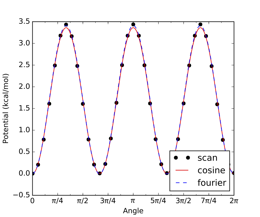
Internal rotation of a methyl group is a common example of a hindered rotor with symmetry = 3, such as the one above. As shown, all three minima (and maxima) have identical energies, hence symmetry = 3.

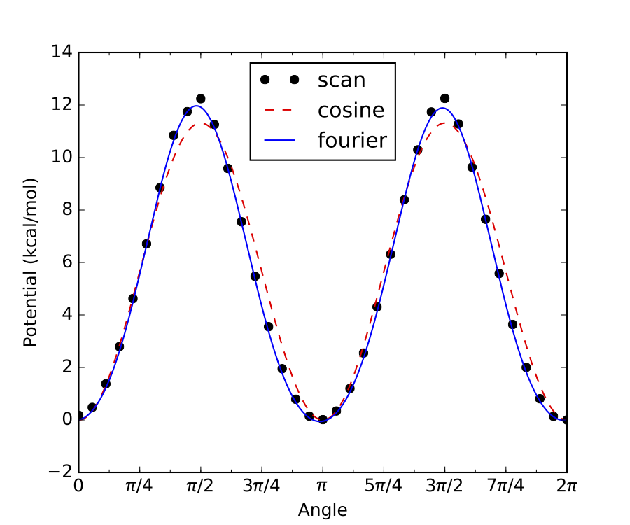
Similarly, if there are only two minima along the internal rotor scan, and both have identical energy, then symmetry = 2, as in the example below:

If any of the energy minima in an internal rotor scan are not identical, then the rotor has no symmetry (symmetry = 1), as in the example below:

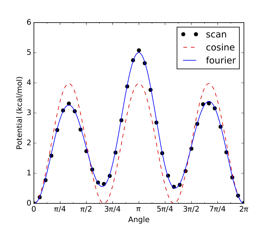
For the example above there are 3 local energy minima, 2 of which are identical to each other. However, the 3rd minima is different from the other 2, therefore this internal rotor has no symmetry.

For practical purposes, when determining the symmetry number for a given hindered rotor simply check if the internal rotor scan looks like the symmetry = 2 or 3 examples above. If it doesn’t, then most likely symmetry = 1.

Each FreeRotor() object requires the following parameters:

Parameter	Description
pivots	The indices of the atoms in the free rotor torsional bond
top	The indices of all atoms on one side of the torsional bond (including the pivot atom)
symmetry	The symmetry number for the torsional rotation (number of indistinguishable energy minima)

Note that a scanLog is not needed for FreeRotor() because it is assumed that there is no barrier to internal rotation. Modeling an internal rotation as a FreeRotor() puts an upper bound on the impact of that rotor on the species’s overall partition function. Modeling the same internal rotation as a Harmonic Oscillator (default if it is not specifed as either a FreeRotor() or HinderedRotor()) puts a lower bound on the impact of that rotor on the species’s overall partition function. Modeling the internal rotation as a HinderedRotor() should fall in between these two extremes.

To summarize, the species input file with hindered/free rotors should look like the following example (different options for specifying the same rotors entry are commented out):

bonds = {
    'C-C': 1,
    'C-H': 6,
}

linear = False

externalSymmetry = 6

spinMultiplicity = 1

opticalIsomers = 1

energy = {
    'CBS-QB3': Log('ethane_cbsqb3.log'),
    'Klip_2': -79.64199436,
}

geometry = Log('ethane_freq.log')

frequencies = Log('ethane_freq.log')

rotors = [
    HinderedRotor(scanLog=Log('ethane_scan_1.log'), pivots=[1,5], top=[1,2,3,4], symmetry=3, fit='best'),
    #HinderedRotor(scanLog=ScanLog('C2H6_rotor_1.txt'), pivots=[1,5], top=[1,2,3,4], symmetry=3, fit='best'),
    #FreeRotor(pivots=[1,5], top=[1,2,3,4], symmetry=3),
]

Note that the atom labels identified within the rotor section should correspond to the indicated geometry.

3.4.1.3. Multidimensional Hindered Rotors

For multidimensional hindered rotors, geometry, frequencies need to be specified in the same way described in detail in the last section. However, rotor files may be specified by either a 1D rotor scan file as in the last section (1D rotors only) or as a directory. The directory must contain a list of energy files in the format something_name_rotorAngle1_rotorAngle2_rotorAngle3(...).log.

For HinderedRotor2D (Quantum Mechanical 2D using Q2DTor):

Parameter	Description
scandir	file or directory containing scan energies
pivots1	The indices of the atoms in the first rotor torsional bond
top1	The indices of all atoms on one side of the first torsional bond (including the pivot atom)
symmetry1	The symmetry number of the first rotor
pivots2	The indices of the atoms in the second rotor torsional bond
top2	The indices of all atoms on one side of the second torsional bond (including the pivot atom)
symmetry2	The symmetry number of the second rotor
symmetry	Q2DTor simplifying symmetry code, default is none

For HinderedRotorClassicalND (Classical and Semiclassical ND rotors):

Parameter	Description
scandir	file or directory containing scan energies
pivots	The list of the indices of the atoms in each rotor torsional bond
tops	The list of the indices of all atoms on one side of each torsional bond (including the pivot atom)
sigmas	The list of symmetry numbers for each torsional bond
semiclassical	Indicates whether to use the semiclassical rotor correction (highly recommended)

The inputs are mostly the same as the last section except that HinderedRotorClassicalND takes lists of pivots, tops and sigmas instead of individual values. These rotor objects enable calculation of partition functions for multidimensional torsions that are particularly important for QOOH molecules and molecules involving intramolecular hydrogen bonding. It is worth noting that HinderedRotor2D can take on the order of hours to run. To mitigate this the .evals file in the directories Q2DTor directories are searched for automatically and used if present to reduce runtime to seconds. This means if you have run a system with HinderedRotor2D and wish to rerun the system and recalculate the HinderedRotor2D you should delete the .evals file. HinderedRotorClassicalND usually runs quickly for lower dimensional torsions.

3.4.1.4. Additional parameters for pressure dependent networks

Additional parameters apply only to molecules in pressure dependent networks

Parameter	Required?	Description
structure	all species except bath gas	A chemical structure for the species defined using either SMILES, adjacencyList, or InChI
molecularWeight	optional for all species	The molecular weight, if not given it is calculated based on the structure
reactive	only bath gases	Boolean indicating whether the molecule reacts, set to False for bath gases. default is True
collisionModel	unimolecular isomers and bath gases	Transport data for the species
energyTransferModel	unimolecular isomers	Assigned with SingleExponentialDown model

The structure parameter is defined by SMILES, adjList, or InChI. For instance, either representation is acceptable for the acetone molecule:

structure = SMILES('CC(C)=O')

structure = adjacencyList("""1  C u0 p0 c0 {2,S} {5,S} {6,S} {7,S}
                             2  C u0 p0 c0 {1,S} {3,S} {4,D}
                             3  C u0 p0 c0 {2,S} {8,S} {9,S} {10,S}
                             4  O u0 p2 c0 {2,D}
                             5  H u0 p0 c0 {1,S}
                             6  H u0 p0 c0 {1,S}
                             7  H u0 p0 c0 {1,S}
                             8  H u0 p0 c0 {3,S}
                             9  H u0 p0 c0 {3,S}
                             10 H u0 p0 c0 {3,S}""")

structure = InChI('InChI=1S/C3H6O/c1-3(2)4/h1-2H3')

The molecularWeight parameter should be defined in the quantity format (value, 'units') , for example:

molecularWeight = (44.04, 'g/mol')

If the molecularWeight parameter is not given, it is calculated by Arkane based on the chemical structure.

The collisionModel is defined for unimolecular isomers with the transport data using a TransportData object:

collisionModel = TransportData(sigma=(3.70,'angstrom'), epsilon=(94.9,'K'))

sigma and epsilon are Lennard-Jones parameters, which can be estimated using the Joback method on the RMG website.

The energyTransferModel model available is a SingleExponentialDown.

• SingleExponentialDown - Specify alpha0, T0 and n for the average energy transferred in a deactiving collision

  \[\left< \Delta E_\mathrm{down} \right> = \alpha_0 \left( \frac{T}{T_0} \right)^n\]

An example of a typical energyTransferModel function is:

energyTransferModel = SingleExponentialDown(
        alpha0 = (0.5718,'kcal/mol'),
        T0 = (300,'K'),
        n = 0.85,
    )

Parameters for the single exponential down model of collisional energy transfer are usually obtained from analogous systems in literature. For example, if the user is interested in a pressure-dependent network with overall molecular formula C7H8, the single exponential down parameters for toluene in helium availabe from literature could be used for all unimolecular isomers in the network (assuming helium is the bath gas). One helpful literature source for calculated exponential down parameters is the following paper: http://www.sciencedirect.com/science/article/pii/S1540748914001084#s0060

3.4.2. Option #2: Directly Enter Molecular Properties

While it is usually more convenient to have Arkane parse molecular properties from the output of quantum chemistry calculations (see Option #1: Automatically Parse Quantum Chemistry Calculation Output) there are instances where an output file is not available and it is more convenient for the user to directly enter the molecular properties. This is the case, for example, if the user would like to use calculations from literature, where the final calculated molecular properties are often reported in a table (e.g., vibrational frequencies, rotational constants), but the actual output files of the underlying quantum chemistry calculations are rarely provided.

For this option, there are a number of required parameters associated with the species() function

Parameter	Required?	Description
label	yes	A unique string label used as an identifier
E0	yes	The ground-state 0 K enthalpy of formation (including zero-point energy)
modes	yes	The molecular degrees of freedom (see below)
spinMultiplicity	yes	The ground-state spin multiplicity (degeneracy), sets to 1 by default if not used
opticalIsomers	yes	The number of optical isomers of the species, sets to 1 by default if not used

The label parameter should be set to a string with the desired name for the species, which can be reference later in the input file.

label = 'C2H6'

The E0 ground state 0 K enthalpy of formation (including zero-point energy) should be given in the quantity format (value, 'units'), using units of either kJ/mol, kcal/mol, J/mol, or cal/mol:

E0 = (100.725, 'kJ/mol')

Note that if Arkane is being used to calculate the thermochemistry of the species, it is critical that the value of E0 is consistent with the definition above (0 K enthalpy of formation with zero-point energy). However, if the user is only interested in kinetics, E0 can be defined on any arbitrary absolute energy scale, as long as the correct relative energies between various species() and transitionState() are maintained. For example, it is common in literature for the energy of some reactant(s) to be arbitrarily defined as zero, and the energies of all transition states, intermediates and products are reported relative to that.

Also note that the value of E0 provided here will be used directly, i.e., no atom or bond corrections will be applied.

If you want Arkane to correct for zero point energy, you can either just place the raw units in Hartree (as if it were read directly from quantum):

E0 = 547.6789753223456

Or you can add a third argument to the Quantity specified whether zero-point energy is included or not:

E0 = (95.1, 'kJ/mol', 'e_electronic')  # when zero point energy (ZPE) is not included - Arkane will add it
E0 = (95.1, 'kJ/mol', 'E0')  # when ZPE is already included - Arkane will not add it

When specifying the modes parameter, define a list with the following types of degrees of freedom. To understand how to define these degrees of freedom, please click on the links below:

Translational degrees of freedom

Class	Description
IdealGasTranslation	A model of three-dimensional translation of an ideal gas

Rotational degrees of freedom

Class	Description
LinearRotor	A model of two-dimensional rigid rotation of a linear molecule
NonlinearRotor	A model of three-dimensional rigid rotation of a nonlinear molecule
KRotor	A model of one-dimensional rigid rotation of a K-rotor
SphericalTopRotor	A model of three-dimensional rigid rotation of a spherical top molecule

Vibrational degrees of freedom

Class	Description
HarmonicOscillator	A model of a set of one-dimensional harmonic oscillators

Note that the frequencies provided here will be used directly, i.e., the frequencyScaleFactor will not be applied.

Torsional degrees of freedom

Class	Description
HinderedRotor	A model of a one-dimensional hindered rotation
FreeRotor	A model of a one-dimensional free rotation

The spinMultiplicity is defined using an integer, and is set to 1 if not indicated in the species() function.

spinMultiplicity = 1

Similarly, the opticalIsomers is also defined using an integer, and is set to 1 if not used in the species() function.

opticalIsomers = 1

The following is an example of a typical species() function, based on ethane (different options for specifying the same internal rotation are commented out):

species(
    label = 'C2H6',
    E0 = (100.725, 'kJ/mol'),
    modes = [
        IdealGasTranslation(mass=(30.0469, 'amu')),
        NonlinearRotor(
            inertia = ([6.27071, 25.3832, 25.3833], 'amu*angstrom^2'),
            symmetry = 6,
        ),
        HarmonicOscillator(
            frequencies = ([818.917, 819.48, 987.099, 1206.81, 1207.06, 1396, 1411.35, 1489.78, 1489.97, 1492.49, 1492.66, 2995.36, 2996.06, 3040.83, 3041, 3065.86, 3066.02], 'cm^-1'),
        ),
        HinderedRotor(
            inertia = (1.56768, 'amu*angstrom^2'),
            symmetry = 3,
            barrier = (11.2717, 'kJ/mol'),
        ),
        #HinderedRotor(
        #inertia = (1.56768, 'amu*angstrom^2'),
        #symmetry = 3,
        #fourier = (
        #    [
        #        [0.00458375, 0.000841648, -5.70271, 0.00602657, 0.0047446],
        #        [0.000726951, -0.000677255, 0.000207033, 0.000553307, -0.000503303],
        #    ],
        #    'kJ/mol',
        #),
        #),
        #FreeRotor(
        #    inertia = (1.56768, 'amu*angstrom^2'),
        #    symmetry = 3,
        #),
    ],
    spinMultiplicity = 1,
    opticalIsomers = 1,
)

Note that the format of the species() function above is identical to the conformer() function output by Arkane in output.py. Therefore, the user could directly copy the conformer() output of an Arkane job to another Arkane input file, change the name of the function to species() (or transitionState(), if appropriate, see next section) and run a new Arkane job in this manner. This can be useful if the user wants to easily switch a species() function from Option #1: Automatically Parse Quantum Chemistry Calculation Output to Option #2: Directly Enter Molecular Properties.

3.4.2.1. Additional parameters for pressure dependent networks

Additional parameters apply only to molecules in pressure depedent networks

Parameter	Required?	Description
structure	all species except bath gas	A chemical structure for the species defined using either SMILES, adjacencyList, or InChI
reactive	only bath gases	Boolean indicating whether the molecule reacts, set to False for bath gases. default is True
collisionModel	unimolecular isomers and bath gases	Transport data for the species
energyTransferModel	unimolecular isomers	Assigned with SingleExponentialDown model
thermo	optional	Thermo data for the species

The parameters structure, molecularWeight, collisionModel and energyTransferModel were already discussed above in Option #1: Automatically Parse Quantum Chemistry Calculation Output.

When the thermo parameter is specified, Arkane will approximate the modes of vibration and energy from the thermodynamic parameters, and will utilize this in its solution of the pressure dependent network. This is analygous to how RMG calculates thermodynamic parameters for pressure dependent mechanisms.

The thermo parameter has the following synatx:

thermo = NASA(polynomials=[
                    NASAPolynomial(coeffs=[3.81543,0.0114632,0.000281868,
                                     -5.70609e-07,3.57113e-10,45814.7,14.9594],
                              Tmin=(10,'K'), Tmax=(510.16,'K')),
                    NASAPolynomial(coeffs=[-1.32176,0.0893697,-5.78295e-05,
                                     1.78722e-08,-2.11223e-12,45849.2,31.4869],
                              Tmin=(510.16,'K'), Tmax=(3000,'K'))
                          ],
              Tmin=(10,'K'), Tmax=(3000,'K')),

3.4.3. Option #3: Automatically Parse YAML files

Arkane automatically saves a .yml file representing an ArkaneSpecies in an ArkaneSpecies folder under the run directory with the statistical mechanics properties of a species along with additional useful metadata. This process is triggered whenever a thermo calculation is ran for a species with a specified structure. To automatically generate such file in the first place, a species has to be defined using one of the other options above. The generated .yml file could conveniently be used when referring to this species in subsequent Arkane jobs. We intend to create an online repository of Arkane .yml files, from which users would be able to pick the desired species calculated at an appropriate level of theory (if available), and directly use them for kinetic or pressure-dependent calculations. Once such repository becomes available, a full description will be added to these pages.

3.5. Transition State

Transition state(s) are only required when performing kinetics computations. Each transition state of interest must be specified using a transitionState() function, which is analogous to the species() function described above. Therefore, the transitionState() function may also be specified in two ways: Option #1: Automatically Parse Quantum Chemistry Calculation Output and Option #2: Directly Enter Molecular Properties. Note that currently a transitions state cannot be specified using a YAML file (Option #3).

The following is an example of a typical transitionState() function using Option #1:

transitionState('TS', 'TS.py')

Just as for a species() function, the first parameter is the label for that transition state, and the second parameter points to the location of another python file containing details of the transition state. This file will be referred to as the transition state input file, and it accepts the same parameters as the species input file described in Option #1: Automatically Parse Quantum Chemistry Calculation Output.

The following is an example of a typical transitionState() function using Option #2:

transitionState(
    label = 'TS',
    E0 = (267.403, 'kJ/mol'),
    modes = [
        IdealGasTranslation(mass=(29.0391, 'amu')),
        NonlinearRotor(
            inertia = ([6.78512, 22.1437, 22.2114], 'amu*angstrom^2'),
            symmetry = 1,
        ),
        HarmonicOscillator(
            frequencies = ([412.75, 415.206, 821.495, 924.44, 982.714, 1024.16, 1224.21, 1326.36, 1455.06, 1600.35, 3101.46, 3110.55, 3175.34, 3201.88], 'cm^-1'),
        ),
    ],
    spinMultiplicity = 2,
    opticalIsomers = 1,
    frequency = (-750.232, 'cm^-1'),
)

The only additional parameter required for a transitionState() function as compared to a species() function is frequency, which is the imaginary frequency of the transition state needed to account for tunneling. Refer to Option #2: Directly Enter Molecular Properties for a more detailed description of the other parameters.

3.6. Reaction

This is only required if you wish to perform a kinetics computation. Each reaction of interest must be specified using a reaction() function, which accepts the following parameters:

Parameter	Required?	Description
label	All reactions	A name for the reaction
reactants	All reactions	A list of reactant species
products	All reactions	A list of product species
transitionState	All reactions	The transition state
kinetics	Optional	The high pressure-limit kinetics for the reaction, for pdep calculations
tunneling	Optional	The type of tunneling model (either ‘Eckhart’ or ‘Wigner’) to use for tunneling through the reaction barrier

The following is an example of a typical reaction function:

reaction(
    label = 'H + C2H4 <=> C2H5',
    reactants = ['H', 'C2H4'],
    products = ['C2H5'],
    transitionState = 'TS',
    tunneling='Eckart'
)

Note that the reactants and products must have been previously declared using a species() function, using the same name labels. Transition states must also be previously declared using a transitionState() function. The quantum tunneling factor method that may be assigned is either 'Eckart' or 'Wigner'.

The kinetics parameter is only useful in pressure dependent calculations. If the optional kinetics parameter is specified, Arkane will perform an inverse Laplace transform (ILT) on the high pressure-limit kinetics provided to estimate the microcanonical rate coefficients, \(k(E)\), needed for the master equation (refer to Theory manual for more detail). This feature is useful for barrierless reactions, such as radical recombinations, which don’t have an obvious transition state. If the ILT approach to calculating \(k(E)\) is taken, a placeholder transitionState must still be defined with an E0 equal to the energy of the higher energy species it is connecting. If the optional kinetics entry is not specified, Arkane will calculate the required kinetic coefficients on its own. The kinetics entry is particularly useful to specify rates of barrierless reactions (for which Arkane cannot yet calculate high-pressure limit rates). The kinetics argument has the following syntax:

kinetics = Arrhenius(A=(2.65e6,'m^3/(mol*s)'), n=0.0, Ea=(0.0,'kcal/mol'), T0=(1,"K")),

For high pressure limit kinetics calculations, specifying the kinetics parameter will just output the value specified by the kinetics parameter, without using transition state theory.

3.7. Thermodynamics

Use a thermo() function to make Arkane execute the thermodynamic parameters computatiom for a species. Pass the string label of the species you wish to compute the thermodynamic parameters for and the type of thermodynamics polynomial to generate (either 'Wilhoit' or 'NASA'). A table of relevant thermodynamic parameters will also be displayed in the output file.

Below is a typical thermo() execution function:

thermo('ethane', 'NASA')

3.8. High Pressure Limit Kinetics

Use a kinetics() function to make Arkane execute the high-pressure limit kinetic parameters computation for a reaction. The 'label' string must correspond to that of a defined reaction() function.

By default, Arkane outputs high pressure kinetic rate coefficients in the modified three-parameter Arrhenius equation format:

\[k(T) = A \left( \frac{T}{T_0} \right)^n \exp \left( -\frac{E_a}{RT} \right)\]

Alternatively, the user may request to output the rate in the classical two-parameter Arrhenius format:

\[k(T) = A \exp \left( -\frac{E_a}{RT} \right)\]

by passing three_params = False in the kinetics() function:

kinetics(
label = 'H + C2H4 <=> C2H5',
three_params = False,
)

You have three options for specifying the temperature to which a modified/classical Arrhenius expression will be fit.

Give an explicit list of temperatures to fit:

kinetics(
label = 'H + C2H4 <=> C2H5',
Tlist = ([400,500,700,900,1100,1200],'K'),
)

Give minimmum and maximum temperatures to fit:

kinetics(
label = 'H + C2H4 <=> C2H5',
Tmin = (400,'K'), Tmax = (1200,'K'), Tcount = 6,
)

Use the default range to fit (298 K to 2500 K at 50 points spaced equally in 1/T space):

kinetics(label = 'H + C2H4 <=> C2H5')

If a sensitivity analysis is desired, simply add the conditions at which to calculate sensitivity coefficients in the following format, e.g.:

kinetics(
    label = 'HSOO <=> HOOS',
    Tmin = (500,'K'), Tmax = (3000,'K'), Tcount = 15,
    sensitivity_conditions = [(1000, 'K'), (2000, 'K')]
)

The output.py file will show the rates at various temperatures including the quantum tunneling factor. Kinetic rates will also be added to the chem.inp file.

The output of a sensitivity analysis is saved into a sensitivity folder in the output directory. A text file, named with the reaction label, delineates the semi-normalized sensitivity coefficients dln(k)/dE0 in units of mol/J at all requested conditions. A horizontal bar figure is automatically generated per reaction with subplots for both the forward and reverse direction at all conditions.

3.9. Pressure Dependent Network Specification

To obtain pressure dependent rates, you need to add two different sections to the file. First, a declaration for the overall network must be given using the network() function, which specifies which spiecies are contained in this reaction network. After that you will need to create a pressureDependence() block that indicates how the pressure dependence calculation should be conducted.

This section will go over the first of these sections, the network() function. This includes setting the following paramters:

Parameter	Description
label	A name for the network
isomers	A list of species participating in unimolecular reaction channels
reactants	A list of the species that participate in bimolecular reactant channels
bathGas	A dictionary of bath gases and their respective mole fractions, adding up to 1.0

Arkane is largely able to determine the molecular configurations that define the potential energy surface for your reaction network simply by inspecting the path reactions. However, you must indicate which unimolecular and bimolecular configurations you wish to include in the master equation formulation; all others will be treated as irreversible sinks.

Note that all species and bath gases used in the network function must have been previously declared with the same name labels in a previous species function in the input file.

You do not need to specify the product channels (infinite sinks) in this manner, as any configuration not marked as an isomer or reactant channel will be treated as a product channel.

An example of the network function is given below along with a scheme of the network:

network(
    label = 'acetyl + O2',
    isomers = [
        'acetylperoxy',
        'hydroperoxylvinoxy',
    ],
    reactants = [
        ('acetyl', 'oxygen'),
    ],
    bathGas = {
        'nitrogen': 0.4,
        'argon': 0.6,
    }
)

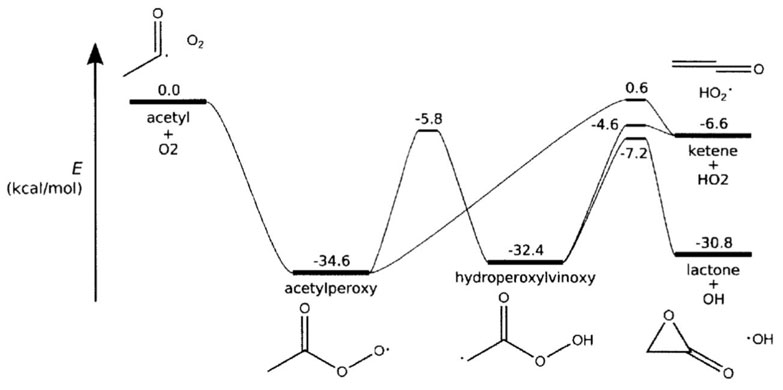
Image source: J.W. Allen, PhD dissertation, MIT 2013, calculated at the RQCISD(T)/CBS//B3LYP/6-311++G(d,p) level of theory

3.10. Pressure Dependent Rate Calculation

The overall parameters for the pressure-dependence calculation must be defined in a pressureDependence() function at the end of the input file. The parameters are:

Parameter	Required?	Description
label	Yes	Use the name for the network declared previously
method	Yes	Method to use for calculating the pdep network. Use either 'modified strong collision', 'reservoir state', or 'chemically-significant eigenvalues'
interpolationModel	Yes	Select the output type for the pdep kinetics, either in 'chebyshev' or 'pdeparrhenius' (plog) format
activeKRotor	No	A flag indicating whether to treat the K-rotor as active or adiabatic (default True)
activeJRotor	No	A flag indicating whether to treat the J-rotor as active or adiabatic (default True)
Tmin/Tmax/Tcount or Tlist	Yes	Define temperatures at which to compute (and output) \(k(T,P)\)
Pmin/Pmax/Pcount or Plist	Yes	Define pressures at which to compute (and output) \(k(T,P)\)
maximumGrainSize	Yes	Defines the upper bound on grain spacing in master equation calculations.
minimumGrainCount	Yes	Defines the minimum number of grains in master equation calculation.
sensitivity_conditions	No	Specifies the conditions at which to run a network sensitivity analysis.

An example of the Pressure-dependent algorithm parameters function for the acetyl + O2 network is shown below:

pressureDependence(
    label='acetyl + O2',
    Tmin=(300.0,'K'), Tmax=(2000.0,'K'), Tcount=8,
    Pmin=(0.01,'bar'), Pmax=(100.0,'bar'), Pcount=5,
    #Tlist = ([300, 400, 600, 800, 1000, 1250, 1500, 1750, 2000],'K')
    #Plist = ([0.01, 0.1, 1.0, 10.0, 100.0],'bar')
    maximumGrainSize = (1.0,'kcal/mol'),
    minimumGrainCount = 250,
    method = 'modified strong collision',
    #method = 'reservoir state',
    #method = 'chemically-significant eigenvalues',
    interpolationModel = ('chebyshev', 6, 4),
    #interpolationModel = ('pdeparrhenius'),
    #activeKRotor = True,
    activeJRotor = True,
    sensitivity_conditions = [[(1000, 'K'), (1, 'bar')], [(1500, 'K'), (10, 'bar')]]
)

3.10.1. Temperature and Pressure Ranges

Arkane will compute the \(k(T,P)\) values on a grid of temperature and pressure points. Tmin, Tmax, and Tcount values, as well as Pmin, Pmax, and Pcount parameter values must be provided. Arkane will automatically choose the intermediate temperatures based on the interpolation model you wish to fit. This is the recommended approach.

Alternatively, the grid of temperature and pressure points can be specified explicitly using Tlist and/or Plist.

3.10.2. Energy Grains

Determine the fineness of the energy grains to be used in the master equation calculations. Dictate the maximumGrainSize, and the minimumGrainCount.

3.10.3. Sensitivity analysis

Arkane also has the ability to vary barrier heights and generate sensitivity coefficients as a function of changes in E0 with the sensitivity_conditions argument. For each desired condition, place its corresponding temperature and pressure within the list of sensitivity_conditions. See the example above for syntax.

The output of a sensitivity analysis is saved into a sensitivity folder in the output directory. A text file, named with the network label, delineates the semi-normalized sensitivity coefficients dln(k)/dE0 in units of mol/J for all network reactions (both directions if reversible) at all requested conditions. Horizontal bar figures are automatically generated per network reaction, showing the semi-normalized sensitivity coefficients at all conditions.

3.11. Atom Energy Fitting

Atom energies can be fitted using a small selection of species (see SPECIES_LABELS in arkane/encorr/ae.py). To do this, the single-point electronic energies calculated using the experimental geometries from the reference database of each of the species should be provided as a dictionary of the species labels and their energies in Hartree. Zero-point energies should not be included in the electronic energies. Each atom energy fitting calculation must be specified using a ae() function, which accepts the following parameters:

Parameter	Required?	Description
species_energies	Yes	Dictionary of species labels and single-point energies
level_of_theory	No	Level of theory used as key if writing to the database dictionary
write_to_database	No	Write the atom energies to the database; requires level_of_theory (default: False)
overwrite	No	If atom energies already exist, overwrite them (default: False)

3.12. Bond Additivity Correction Fitting

If calculated data is available in the reference database, Arkane can fit and save bond additivity corrections (BACs). There are two different types available: Petersson-type (Petersson et al., J. Chem. Phys. 1998, 109, 10570-10579), which fits one parameter for each bond type, and Melius-type (Anantharaman and Melius, J. Phys. Chem. A 2005, 109, 1734-1747), which fits three parameters per atom type and an optional molecular parameter. Each BAC fitting calculation must be specified using a bac() function, which accepts the following parameters:

Parameter	Required?	Description
level_of_theory	Yes	Calculated data will be extracted from the reference database using this level of theory
bac_type	No	BAC type: ‘p’ for Petersson (default), ‘m’ for Melius
train_names	No	Names of training data folders in the RMG database (default: ‘main’)
crossval_n_folds	No	If 1, perform no cross-validation. If -1, perform leave-one-out cross-validation. If any other positive integer, perfrom k-fold cross-validation. (default: 1)
idxs	No	Only include reference species with these indices in the training data (default: None)
exclude_idxs	No	Exclude reference species with these indices from the training data (default: None)
exclude_elements	No	Exclude molecules with the elements in this list from the training data (default: None)
charge	No	Set the allowed charges (‘neutral’, ‘positive’, ‘negative’, or integers) for molecules in the training data (default: ‘all’)
multiplicity	No	Set the allowed multiplicities for molecules in the training data (default: ‘all’)
weighted	No	Weight the data to diversify substructures (default: False)
write_to_database	No	Write the BACs to the database; has no effect if doing cross-validation (default: False)
overwrite	No	If BACs already exist, overwrite them (default: False)
fit_mol_corr	No	Fit the optional molecular correction term (Melius only, default: True)
global_opt	No	Perform a global optimization (Melius only, default: True)
global_opt_iter	No	Number of global optimization iterations (Melius only, default: 10)

3.13. Examples

Perhaps the best way to learn the input file syntax is by example. To that end, a number of example input files and their corresponding output have been given in the examples/arkane directory.

3.14. Troubleshooting and FAQs

1) The network that Arkane generated and the resulting pdf file show abnormally large absolute values. What’s going on?

This can happen if the number of atoms and atom types is not properly defined or consistent in your input file(s).

3.15. Arkane User Checklist

Using Arkane, or any rate theory package for that matter, requires careful consideration and management of a large amount of data, files, and input parameters. As a result, it is easy to make a mistake somewhere. This checklist was made to minimize such mistakes for users:

• Do correct paths exist for pointing to the files containing the electronic energies, molecular geometries and vibrational frequencies?

For calculations involving pressure dependence:

• Does the network pdf look reasonable? That is, are the relative energies what you expect based on the input?

For calculations using internal hindered rotors:

• Did you check to make sure the rotor has a reasonable potential (e.g., visually inspect the automatically generated rotor pdf files)?

• Within your input files, do all specified rotors point to the correct files?

• Do all of the atom label indices correspond to those in the file that is read by Log?

• Why do the fourier fits look so much different than the results of the ab initio potential energy scan calculations? This is likely because the initial scan energy is not at a minimum. One solution is to simply shift the potential with respect to angle so that it starts at zero and, instead of having Arkane read a Qchem or Gaussian output file, have Arkane point to a ‘ScanLog’ file. Another problem can arise when the potential at 2*pi is also not [close] to zero.