15. Liquid Phase Systems

To simulate liquids in RMG requires a module in your input file for liquid-phase:

solvation(
    solvent='octane'
)

Your reaction system will also be different (liquidReactor rather than simpleReactor):

liquidReactor(
    temperature=(500,'K'),
    initialConcentrations={
        "octane": (6.154e-3,'mol/cm^3'),
        "oxygen": (4.953e-6,'mol/cm^3')
    },
    terminationTime=(5,'s'),
    constantSpecies=['oxygen'],
    sensitivity=['octane','oxygen'],
    sensitivityThreshold=0.001,

)

To simulate the liquidReactor, one of the initial species / concentrations must be the solvent. If the solvent species does not appear as the initial species, RMG run will stop and raise error. The solvent can be either reactive, or nonreactive.

In order for RMG to recognize the species as the solvent, it is important to use the latest version of the RMG-database, whose solvent library contains solvent SMILES. If the latest database is used, RMG can determine whether the species is the solvent by looking at its molecular structure (SMILES or adjacency list). If the old version of RMG-database without the solvent SMILES is used, then RMG can recognize the species as the solvent only by its string name. This means that if the solvent is named “octane” in the solvation block and it is named “n-octane” in the species and initialConcentrations blocks, RMG will not be able to recognize them as the same solvent species and raise error because the solvent is not listed as one of the initial species.

For liquid phase generation, you can provide a list of species for which one concentration is held constant over time (Use the keyword constantSpecies=[] with species labels separated by ","). To generate meaningful liquid phase oxidation mechanism, it is highly recommended to consider O2 as a constant species. To consider pyrolysis cases, it is still possible to obtain a mechanism without this option. Expected results with Constant concentration option can be summarized with those 3 cases respectively presenting a generation with 0, 1 (oxygen only) and 2 constant species (oxygen and decane):

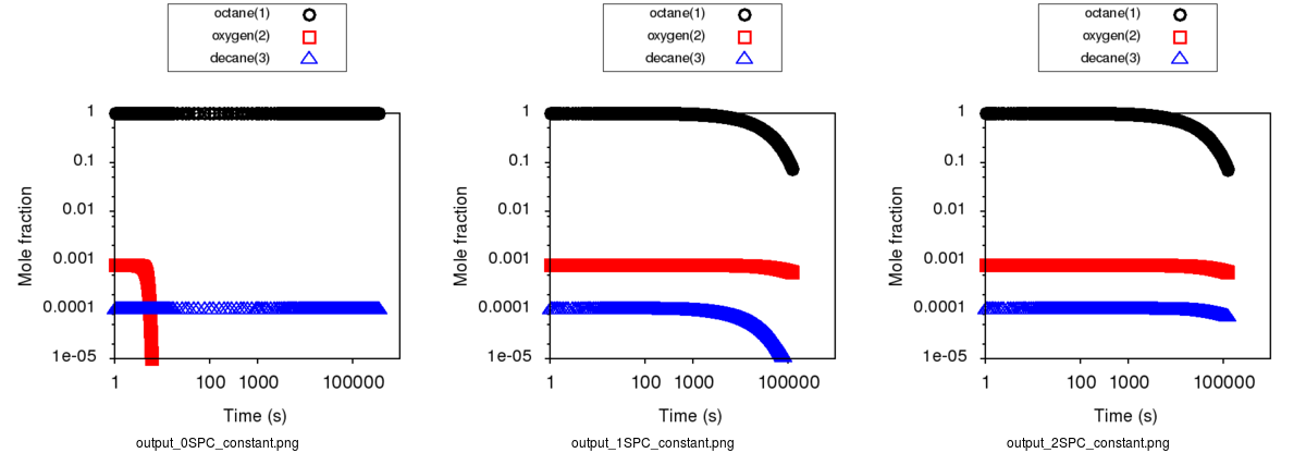
As it creates a mass lost, it is recommended to avoid to put any products as a constant species.

For sensitivity analysis, RMG-Py must be compiled with the DASPK solver, which is done by default but has some dependency restrictions. (See License Restrictions on Dependencies for more details.) Like for the simpleReactor, the sensitivity and sensitivityThrehold are optional arguments for when the user would like to conduct sensitivity analysis with respect to the reaction rate coefficients for the list of species given for sensitivity.

Sensitivity analysis is conducted for the list of species given for sensitivity argument in the input file. The normalized concentration sensitivities with respect to the reaction rate coefficients dln(C_i)/dln(k_j) are saved to a csv file with the file name sensitivity_1_SPC_1.csv with the first index value indicating the reactor system and the second naming the index of the species the sensitivity analysis is conducted for. Sensitivities to thermo of individual species is also saved as semi normalized sensitivities dln(C_i)/d(G_j) where the units are given in 1/(kcal mol-1). The sensitivityThreshold is set to some value so that only sensitivities for dln(C_i)/dln(k_j) > sensitivityThreshold or dlnC_i/d(G_j) > sensitivityThreshold are saved to this file.

Note that in the RMG job, after the model has been generated to completion, sensitivity analysis will be conducted in one final simulation (sensitivity is not performed in intermediate iterations of the job).

Notes: sensitivity, sensitivityThreshold and constantSpecies are optionnal keywords.

15.1. Equation of state

Specifying a liquidReactor will have two effects:

1. disable the ideal gas law renormalization and instead rely on the concentrations you specified in the input file to initialize the system.

2. prevent the volume from changing when there is a net stoichiometry change due to a chemical reaction (A = B + C).

15.2. Solvation thermochemistry

The next correction for liquids is solvation effects on the thermochemistry. By specifying a solvent in the input file, we load the solvent parameters to use.

The free energy change associated with the process of transferring a molecule from the gas phase to the solvent phase at constant \(T\) and \(P\) is defined as the free energy of solvation. Commonly, the standard state of the ideal gas and ideal solution at equal and dilute solute concentrations, also known as the Ben-Naim standard state, is used for solvation free energy (\(\Delta G_{\rm solv}^{*}\)) [BenNaim1987]. Solvation energy is added to the gas phase Gibbs free energy as a correction to estimate the free energy of the compound in a liquid phase:

(1)\[\Delta G_{\rm liquid}^{*} \approx \Delta G_{\rm f, gas}^{\circ} + \Delta G_{\rm solv}^{*}\]

Many different methods have been developed for computing solvation energies among which continuum dielectric and force field based methods are popular. Not all of these methods are easy to automate, and many are not robust i.e. they either fail or give unreasonable results for certain solute-solvent pairs. CPU time and memory (RAM) requirements are also important considerations. A fairly accurate and fast method for computing \(\Delta G_{\rm solv}^{*}\), which is used in RMG, is the LSER approach described below.

15.2.1. Use of thermo libraries in liquid phase system

As it is for gas phase simulation, thermo libraries listed in the input files are checked first to find thermo for a given species and return the first match. As it exists two types of thermo libraries, (more details on thermo libraries), thermo of species matching a library in a liquid phase simulation is obtained following those two cases:

If library is a “liquid thermo library”, thermo data are directly used without applying solvation on it.

If library is a “gas thermo library”, thermo data are extracted and then corrections are applied on it using the LSER method for this specific species-solvent system.

Note

Gas phase libraries can be declared first, liquid thermo libraries will still be tested first but the order will be respected if several liquid libraries are provided.

15.2.2. Use of Abraham LSER to estimate thermochemistry at 298 K

The Abraham LSER provides an estimate of the the partition coefficient (\(K\)) of a solute (component 2) between the vapor phase and a particular solvent (component 1) at 298 K:

(2)\[\log_{10} K = c + eE + sS + aA + bB + lL\]

where the partition coefficient is the ratio of the equilibrium concentrations of the solute in liquid and vapor phases

(3)\[K = \frac{c_{\rm 2, liquid}}{c_{\rm 2, gas}}\]

The Abraham model is used in RMG to estimate \(\Delta G_{\rm solv}^{*}\) which is related to the \(K\) of a solute according to the following expression:

(4)\[\begin{split}\Delta G_{\rm solv}^{*}({\rm 298 K}) = -RT \ln K \\ = -2.303RT \log_{10} K\end{split}\]

The variables in the Abraham model represent solute (E, S, A, B, V, L) and solvent descriptors (c, e, s, a, b, v, l) for different interactions. The sS term is attributed to electrostatic interactions between the solute and the solvent (dipole-dipole interactions related to solvent dipolarity and the dipole-induced dipole interactions related to the polarizability of the solvent) [Vitha2006], [Abraham1999], [Jalan2010]. The lL term accounts for the contribution from cavity formation and dispersion (dispersion interactions are known to scale with solute volume [Vitha2006], [Abraham1999]. The eE term, like the sS term, accounts for residual contributions from dipolarity/polarizability related interactions for solutes whose blend of dipolarity/polarizability differs from that implicitly built into the S parameter [Vitha2006], [Abraham1999], [Jalan2010]. The aA and bB terms account for the contribution of hydrogen bonding between the solute and the surrounding solvent molecules. H-bonding interactions require two terms as the solute (or solvent) can act as acceptor (donor) and vice versa. The descriptor A is a measure of the solute’s ability to donate a hydrogen bond (acidity) and the solvent descriptor a is a measure of the solvent’s ability to accept a hydrogen bond. A similar explanation applies to the bB term [Vitha2006], [Abraham1999], [Poole2009].

The enthalpy change associated with solvation at 298 K can be calculated from the Mintz LSER. Mintz et al. ([Mintz2007], [Mintz2007a], [Mintz2007b], [Mintz2007c], [Mintz2007d], [Mintz2008], [Mintz2008a], [Mintz2009]) have developed a linear correlation similar to the Abraham model for estimating \(\Delta H_{\rm solv}^{*}\):

(5)\[\Delta H_{\rm solv}^{*}({\rm 298 K}) = c' + a'A+ b'B+ e'E+ s'S+ l'L\]

where A, B, E, S and L are the same solute descriptors used in the Abraham model for the estimation of \(\Delta G_{\rm solv}^{*}\). The lowercase coefficients c’, a’, b’, e’, s’ and l’ depend only on the solvent and were obtained by fitting to experimental data.

RMG’s database has a solute library that contains the solute descriptors of around 300 compounds and it is located at RMG-database/input/solvation/libraries/solute.py in RMG-database. For the compounds that are not found in the solute library, the group additivity method is used to estimate the solute descriptors as described below under Group additivity method for solute descriptor estimation.

The solvent descriptors (c, e, s, a, b, l, c’, a’, b’, e’, s’, l’) are largely treated as regressed empirical coefficients. The solvent descriptors are fitted by Chung et al. ([Chung2021]) using experimental solute parameter, solvation free energy, and solvation enthalpy data collected from various sources. The Abraham solvent parameters (c, e, s, a, b, v, l) are provided in RMG’s database for 196 pure solvents and 3 binary mixture solvents for solvation free energy calculations. The Mintz solvent parameters (c’, a’, b’, e’, s’) are provided for 69 pure solvents in RMG’s database for solvation enthalpy calculations. A full list of solvents and their solvent parameters can be found on (1) the RMG-database git repository or (2) the RMG website. If RMG-database is installed, these solvent information can be found found in RMG-database/input/solvation/libraries/solvent.py.

You can also search for a solvent by SMILES string using a sample ipython notebook located at RMG-Py/ipython/estimate_solvation_thermo_and_search_available_solvents.ipynb. This ipython notebook takes a SMILES string as an input and checks whether the given compound is found in RMG’s database. It also returns the Abraham and Mintz solvent parameters for the matched solvent. In addition, the ipython notebook shows sample solvation free energy and enthalpy calculations for solute-solvent pairs.

15.2.3. Estimation of \(\Delta G_{\rm solv}^{*}\) at other temperatures: linear extrapolation

To estimate \(\Delta G_{\rm solv}^{*}\) at temperatures other than 298 K, a simple linear extrapolation can be employed. For this approach, the enthalpy and entropy of solvation are assumed to be independent of temperature. The entropy of solvation, \(\Delta S_{\rm solv}^{*}(\rm 298 K)\), is calculated from \(\Delta G_{\rm solv}^{*}(\rm 298 K)\) and \(\Delta H_{\rm solv}^{*}(\rm 298 K)\) estimated from the Abraham and Mintz LSERs.

(6)\[\Delta S_{\rm solv}^{*}({\rm 298 K}) = \frac{\Delta H_{\rm solv}^{*}({\rm 298 K}) - \Delta G_{\rm solv}^{*}({\rm 298 K})}{\rm 298 K}\]

Then \(\Delta G_{\rm solv}^{*}\) at other temperatures is approximated by simple extrapolation assuming linear temperature dependence.

(7)\[\Delta G_{\rm solv}^{*}(T) = \Delta H_{\rm solv}^{*}({\rm 298 K}) - T\Delta S_{\rm solv}^{*}({\rm 298 K})\]

This method provides a rapid, first-order approximation of the temperature dependence of solvation free energy. However, since the actual solvation enthalpy and entropy vary with temperature, this approximation will deviate at temperatures far away from 298 K. Looking at several experimental data, this approximation seems reasonable up to ~ 400 K.

15.2.4. Estimation of \(\Delta G_{\rm solv}^{*}\) at other temperatures: temperature-dependent model

This method uses a piecewise function of K-factor to estimate more accurate temperature dependent solvation free energy. The K-factor at infinite dilution (\(K_{2,1}^{\infty}\)), also known as the vapor-liquid equilibrium ratio, is defined as the ratio of the equilibrium mole fractions of the solute (component 2) in the gas and the liquid phases of the solvent (component 1):

\[K_{2,1}^{\infty} = \frac{y_{2}}{x_{2}}\]

Recently, Chung et al. ([Chung2020]) has shown that the following piecewise function combining two separate correlations ([Japas1989], [Harvey1996]) can accurately predict the K-factor from room temperature up to the critical temperature of the solvent

(8)\[{\rm For}\ \ T \leqslant 0.75T_{\rm c}:\ \ \ \ \ \ \ \ \ T_{\rm r}\ln K_{2,1}^{\infty} = A + B(1-T_{\rm r})^{0.355} + C(T_{\rm r})^{0.59}\exp (1-T_{\rm r})\]

(9)\[{\rm For}\ \ 0.75T_{\rm c} \leqslant T < T_{\rm c}:\ \ \ \ \ \ \ \ \ \ T_{\rm r}\ln K_{2,1}^{\infty} = D(\frac{\rho_{1}^{\rm l}}{\rho_{\rm c, 1}}-1)\]

where \(A, B, C, D\) are empirical parameters unique for each solvent-solute pair, \(T_{\rm c}\) is the critical temperature of the solvent, \(T_{\rm r}\) is the reduced temperature (\(T_{\rm r} = \frac{T}{T_{\rm c}}\)), \(\rho_{1}^{\rm l}\) is the saturated liquid phase density of the solvent, and \(\rho_{\rm c, 1}\) is the critical density of the solvent. The transition temperature, \(0.75T_{\rm c}\), has been empirically chosen. All calculations are performed at the solvent’s saturation pressures such that K-factor is only a function of temperature.

Solvation free energy can be calculated from K-factor from the following relation

(10)\[\Delta G_{\rm solv}^{*} = RT\ln \left(\frac{K_{2,1}^{\infty} \rho_{1}^{\rm g}}{\rho_{1}^{\rm l}}\right)\]

where \(\rho_{1}^{\rm g}\) is the saturated gas phase density of the solvent.

To solve for the four empirical parameters (A, B, C, D), we need four equations. The first two can be obtained by enforcing the continuity in values and temperature gradient of the piecewise function at the transition temperature. The last two can be obtained by making the K-factor value and its temperature gradient at 298 K match with those estimated from the solvation free energy and enthalpy at 298 K. These lead to the following four linearly independent equations to solve:

(11)\[{\rm At\ } T = {\rm 298 K} :\ \ \ \ \ \ \ \ \ \ \ \ \ \ \ \ \ \ \ \ \ \ \ \ A + B(1-T_{\rm r})^{0.355} + C(T_{\rm r})^{0.59}\exp{(1-T_{\rm r})} =T_{\rm r} \ln{K_{2,1}^{\infty}(298\ \rm K)}\]

(12)\[{\rm At\ } T = {\rm 298 K}:\ \ \ \ \ -\frac{0.355B}{T_{\rm c}}(1-T_{\rm r})^{-0.645} + \frac{C\exp{(1-T_{\rm r})}}{T_{\rm c}}\left(0.59(T_{\rm r})^{-0.41} - (T_{\rm r}^{*})^{0.59}\right) = \frac{{\rm d}\left(T_{\rm r} \ln{K_{2,1}^{\infty}}\right)}{{\rm d}T}\Big|_{T=298\ {\rm K}}\]

(13)\[{\rm At\ } T = 0.75T_{\rm c}:\ \ \ \ \ \ \ \ \ \ \ \ \ \ \ \ \ \ \ \ \ \ \ \ \ \ \ \ A + B(1-T_{\rm r})^{0.355} + C(T_{\rm r})^{0.59}\exp{(1-T_{\rm r})} = D\Big(\frac{\rho_{1}^{\rm l}}{\rho_{\rm c,1}} - 1 \Big)\]

(14)\[{\rm At\ } T = 0.75T_{\rm c}:\ \ \ \ \ \ \ \ \ \ \ \ \ -\frac{0.355B}{T_{\rm c}}(1-T_{\rm r})^{-0.645} + \frac{C\exp{(1-T_{\rm r})}}{T_{\rm c}}\left(0.59(T_{\rm r})^{-0.41} - (T_{\rm r})^{0.59}\right) = \frac{D}{\rho_{\rm c, 1}} \frac{{\rm d}\rho_{1}^{\rm l}}{{\rm d}T}\Big|_{T=0.75T_{\rm c}}\]

The temperature dependent liquid phase and gas phase densities of solvents can be evaluated at the solvent’s saturation pressure using CoolProp [Bell2014]. CoolProp is an open source fluid modeling software based on Helmholtz energy equations of state. It provides accurate estimations of fluid properties over the wide ranges of temperature and pressure for a variety of fluids. With known solvents’ densities, one can easily find the empirical parameters of the piecewise functions by solving the linear equations above without using any experimental data.

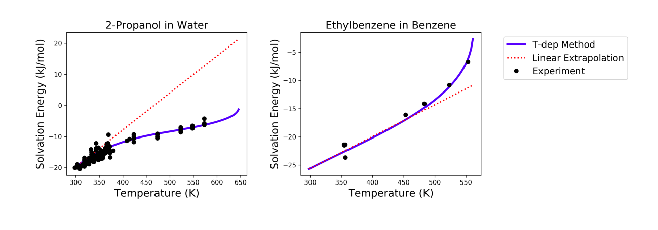
This method has been tested for 47 solvent-solute pairs over a wide range of temperature, and the mean absolute error of solvation free energies has been found to be 1.6 kJ/mol [Chung2020]. Sample plots comparing the predictions made by this temperature dependent method and the linear extrapolation method are shown below. The experimental data are obtained from the Dortmund Databank integrated in SpringerMaterials [DDBST2014].

A sample ipython notebook script for temperature dependent K-factor and solvation free energy calculations can be found under $RMG-Py/ipython/temperature_dependent_solvation_free_energy.ipynb. These calculations are also available on a web browser from the RMG website: Solvation Search.

However not every solvent listed in the RMG solvent database is available in CoolProp. Here is a list of solvents that are available in CoolProp and therefore are available for temperature dependent solvation calculations:

1. benzene

2. cyclohexane

3. decane

4. dichloroethane

5. dodecane

6. ethanol

7. heptane

8. hexane

9. nonane

10. octane

11. pentane

12. toluene

13. undecane

14. water

15.2.5. Current status of temperature dependent \(\Delta G_{\rm solv}^{*}\) in RMG liquid reactor

Currently, RMG uses the linear extrapolation method to estimate solvation free energy at temperatures other than 298 K. The work is in progress to implement the temperature dependent solvation free energy estimation for available solvents.

15.2.6. Group additivity method for solute descriptor estimation

Group additivity or group contribution is a convenient way of estimating the thermochemistry for thousands of species sampled in a typical mechanism generation job. Use of the Abraham Model in RMG requires a similar approach to estimate the solute descriptors (A, B, E, L, and S). RMG uses the group additivity method devised by Chung et al. [Chung2021] for solute descriptor estimation. The solute descriptor group additivity follows the same scheme as the RMG’s group additivity method for gas phase thermochemistry estimation, which is explained in Thermochemistry Estimation and Thermo Database. It estimates the solute descriptors by dividing a molecule into atom-centered (AC) functional groups and summing the contribution from all groups. Additionally, RMG implements ring strain correction (RSC) and long distance interaction (LDI) groups to account for more advanced structural effects that cannot be captured by the atom-based approach. E.g.:

\[E, S, A, B,\ \mathrm{or}\ L = \sum_{i=1}^{N_{\mathrm{atom}}} \mathrm{AC}_{i} + \sum_{j=1} \mathrm{RSC}_{j} + \sum_{k=1} \mathrm{LDI}_{k}\]

where \(N_{\mathrm{atom}}\) is the number of heavy atoms in a molecule and RSC and LDI corrections are applied for each ring cluster and long distance interaction group found in a molecule, respectively.

While most molecules follow the equation above, halogenated molecules are treated differently in RMG for solute descriptor estimation: all halogen atoms are first replaced by hydrogen atoms, then the group additivity estimate is made on the replaced structure, and halogen corrections are lastly added for each halogen atom to get the final prediction as shown below:

\[ \begin{align}\begin{aligned} E, S, A, B,\ \mathrm{or}\ L = \sum_{i=1}^{N_{\mathrm{atom*}}} \mathrm{AC}_{i} + \sum_{j=1} \mathrm{RSC}_{j} + \sum_{k=1} \mathrm{LDI}_{k} + \sum_{l=1}^{N_{\mathrm{halogen}}} \mathrm{Halogen}_{l}\\= (E, S, A, B,\ \mathrm{or}\ L)_{\mathrm{replaced\ compound}} + \sum_{l=1}^{N_{\mathrm{halogen}}} \mathrm{Halogen}_{l}\end{aligned}\end{align} \]

where the subscript ‘replaced compound’ denotes the compound whose halogen atoms are replaced by hydrogen atoms, and \(N_{\mathrm{atom*}}\) and \(N_{\mathrm{halogen}}\) represent the number of non-halogen heavy atoms and the number of halogen atoms in a molecule, respectively. We take this unique approach because it allows one to use the experimental solute parameter data of a replaced compound and simply apply halogen corrections to get more accurate estimates for a halogenated compound.

For radical species, RMG uses the hydrogen bond increment (HBI) method developed by Lay et al. [Lay] to estimate the solute descriptors. The HBI method first saturates the compound, gets the estimate using the saturated structure, and applies the radical corrections for each radical site using the original structure as shown below:

\[E, S, A, B,\ \mathrm{or}\ L = (E, S, A, B,\ \mathrm{or}\ L)_{\mathrm{saturated}} + \sum_{m=1}^{N_{\mathrm{radical}}} \mathrm{radical}_{m}\]

where the subscript ‘saturated’ denotes the compound whose radical sites are saturated and \(N_{\mathrm{radical}}\) is the number of radical sites in a molecule. If the solute descriptors for the saturated structure are available in the RMG-database solute library, the group additivity approach will use the library data and apply the HBI corrections to get the estimates for the radical. If the solute descriptors for the saturated structure are not available in the solute library, RMG will use the group additivity approach to estimate the solute descriptors for the saturated structure and apply the HBI corrections.

If a species is a radical and contains any halogen atoms, RMG’s solute descriptor group additivity method will first saturate the compound and check whether the saturated form can be found in the solute libraries. If yes, it uses the solute data of the saturated form and applies the HBI corrections on the original molecule. If the saturated form cannot be found in the solute libraries, it then replaces the halogen atoms with hydrogen atoms and checks whether the saturated, replaced form can be found in the solute libraries. If yes, it uses the solute data of the saturated, replaced form, applies a halogen correction for each halogenated site on the saturated from, and finally performs the HBI corrections on the original molecule. If the saturated, replaced form cannot be found in the solute libraries, it computes the solute data for the saturated, replaced form using group additivity, applies a halogen correction for each halogenated site on the saturated form, and finally performs the HBI corrections on the original molecule.

A sample ipython script that shows the solute parameter group additivity calculations, solvation free energy and enthalpy calculations can be found at RMG-Py/ipython/estimate_solvation_thermo_and_search_available_solvents.ipynb.

The group contribution databases for the solute descriptors can be found under RMG-database/input/solvation/groups/ in RMG-database. Each particular type of group contribution is stored in a file with the extension .py, e.g. ‘groups.py’:

file	Type of group contribution
group.py	group additive values (ACs)
ring.py	monocyclic ring corrections (RSCs)
polycyclic.py	polycyclic ring corrections (RSCs)
longDistanceInteraction_cyclic.py	aromatic ortho, meta, para correction (LDIs)
longDistanceInteraction_noncyclic.py	gauche interaction correction (LDIs)
halogen.py	halogen corrections (halogens)
radical.py	hydrogen bond increments (HBIs)

Like many other entities in RMG, the database of each type of group contribution is organized in a hierarchical tree, and is defined at the bottom of the database file.

More information on hierarchical tree structures in RMG can be found here: Introduction.

For information on the estimated prediction errors of the group additivity method, please refer to the work by Chung et al. [Chung2021]

15.3. Diffusion-limited kinetics

The next correction for liquid-phase reactions is to ensure that bimolecular reactions do not exceed their diffusion limits. The theory behind diffusive limits in the solution phase for bimolecular reactions is well established ([Rice1985]) and has been extended to reactions of any order ([Flegg2016]). The effective rate constant of a diffusion-limited reaction is given by:

(15)\[k_{\mathrm{eff}} = \frac {k_{\mathrm{diff}} k_{\mathrm{int}}}{k_{\mathrm{diff}} + k_{\mathrm{int}}}\]

where \(k_\mathrm{int}\) is the intrinsic reaction rate, and \(k_\mathrm{diff}\) is the diffusion-limited rate, which is given by:

(16)\[k_{\mathrm{diff}} = \left[\prod_{i=2}^N\hat{D}_i^{3/2}\right]\frac{4\pi^{\alpha+1}}{\Gamma(\alpha)}\left(\frac{\sigma}{\sqrt{\Delta_N}}\right)^{2\alpha}\]

where \(\alpha=(3N-5)/2\) and

(17)\[\hat{D}_i = D_i + \frac{1}{\sum_m^{i-1}D_m^{-1}}\]

(18)\[\Delta_N = \frac{\sum_{i=1}^N D_i^{-1}}{\sum_{i>m}(D_iD_m)^{-1}}\]

\(D_i\) are the individual diffusivities and \(\sigma\) is the Smoluchowski radius, which would usually be fitted to experiment, but RMG approximates it as the sum of molecular radii. RMG uses the McGowan method for estimating radii, and diffusivities are estimated with the Stokes-Einstein equation using experimental solvent viscosities (\(\eta(T)\)):

(19)\[D_{i} = \frac{k_{B}T}{6\pi\,\eta\,r_{i}}\]

(20)\[\sigma = \sum_{i=1}^N r_{i}\]

(21)\[r_{i} = \frac{\left(100\frac{3}{4}\frac{V_{i}}{\pi N_{A}}\right)^{1/3}}{100}\]

where \(k_B\) is the Boltzmann constant, \(N_A\) is the Avogadro number, \(r_i\) is the individual molecular radius in meters, and \(V_i\) is the individual McGowan volume in cm3/mol divided by 100, which is equivalent to the Abraham solute parameter, \(V\).

In a unimolecular to bimolecular reaction, for example, the forward rate constant (\(k_f\)) can be slowed down if the reverse rate (\(k_{r,\mathrm{eff}}\)) is diffusion-limited since the equilibrium constant (\(K_{eq}\)) is not affected by diffusion limitations. In cases where both the forward and the reverse reaction rates are multimolecular, the forward rate coefficients limited in the forward and reverse directions are calculated and the limit with the smaller forward rate coefficient is used.

The viscosity of the solvent is calculated Pa.s using the solvent specified in the command line and a correlation for the viscosity using parameters \(A, B, C, D, E\):

(22)\[\ln \eta = A + \frac{B}{T} + C\log T + DT^E\]

The viscosity parameters (A, B, C, D, E) are provided for 150 pure solvents in RMG’s database, which can be found under (1) the RMG-database git repository or (2) the RMG website. If RMG-database is installed, these viscosity parameters can be found found in RMG-database/input/solvation/libraries/solvent.py.

You can also check whether a compound of interest has viscosity parameters in RMG-database by using a SMILES string and a sample ipython notebook located at RMG-Py/ipython/estimate_solvation_thermo_and_search_available_solvents.ipynb.

To build accurate models of liquid phase chemical reactions you will also want to modify your kinetics libraries or correct gas-phase rates for intrinsic barrier solvation corrections (coming soon).

15.4. Example liquid-phase input file, no constant species

This is an example of an input file for a liquid-phase system:

# Data sources
database(
    thermoLibraries = ['primaryThermoLibrary'],
    reactionLibraries = [],
    seedMechanisms = [],
    kineticsDepositories = ['training'],
    kineticsFamilies = 'default',
    kineticsEstimator = 'rate rules',
)

# List of species
species(
    label='octane',
    reactive=True,
    structure=SMILES("C(CCCCC)CC"),
)

species(
    label='oxygen',
    reactive=True,
    structure=SMILES("[O][O]"),
)

# Reaction systems
liquidReactor(
    temperature=(500,'K'),
    initialConcentrations={
        "octane": (6.154e-3,'mol/cm^3'),
        "oxygen": (4.953e-6,'mol/cm^3')
    },
    terminationTime=(5,'s'),
)

solvation(
    solvent='octane'
)

simulator(
    atol=1e-16,
    rtol=1e-8,
)

model(
    toleranceKeepInEdge=1E-9,
    toleranceMoveToCore=0.01,
    toleranceInterruptSimulation=0.1,
    maximumEdgeSpecies=100000
)

options(
    units='si',
    generateOutputHTML=False,
    generatePlots=False,
    saveSimulationProfiles=True,
)

15.5. Example liquid-phase input file, with constant species

This is an example of an input file for a liquid-phase system with constant species:

# Data sources
database(
    thermoLibraries = ['primaryThermoLibrary'],
    reactionLibraries = [],
    seedMechanisms = [],
    kineticsDepositories = ['training'],
    kineticsFamilies = 'default',
    kineticsEstimator = 'rate rules',
)

# List of species
species(
    label='octane',
    reactive=True,
    structure=SMILES("C(CCCCC)CC"),
)

species(
    label='oxygen',
    reactive=True,
    structure=SMILES("[O][O]"),
)

# Reaction systems
liquidReactor(
    temperature=(500,'K'),
    initialConcentrations={
        "octane": (6.154e-3,'mol/cm^3'),
        "oxygen": (4.953e-6,'mol/cm^3')
    },
    terminationTime=(5,'s'),
    constantSpecies=['oxygen'],
)

solvation(
    solvent='octane'
)

simulator(
    atol=1e-16,
    rtol=1e-8,
)

model(
    toleranceKeepInEdge=1E-9,
    toleranceMoveToCore=0.01,
    toleranceInterruptSimulation=0.1,
    maximumEdgeSpecies=100000
)

options(
    units='si',
    generateOutputHTML=False,
    generatePlots=False,
    saveSimulationProfiles=True,
)

[BenNaim1987]

A. Ben-Naim. “Solvation Thermodynamics.” Plenum Press (1987).

[Vitha2006] (1,2,3,4)

M. Vitha and P.W. Carr. “The chemical interpretation and practice of linear solvation energy relationships in chromatography.” J. Chromatogr. A. 1126(1-2), p. 143-194 (2006).

[Abraham1999] (1,2,3,4)

M.H. Abraham et al. “Correlation and estimation of gas-chloroform and water-chloroformpartition coefficients by a linear free energy relationship method.” J. Pharm. Sci. 88(7), p. 670-679 (1999).

[Jalan2010] (1,2)

A. Jalan et al. “Predicting solvation energies for kinetic modeling.” Annu. Rep.Prog. Chem., Sect. C 106, p. 211-258 (2010).

[Poole2009]

C.F. Poole et al. “Determination of solute descriptors by chromatographic methods.” Anal. Chim. Acta 652(1-2) p. 32-53 (2009).

[Lay]

Lay, T.; Bozzelli, J.; Dean, A.; Ritter, E. J. Phys. Chem. 1995, 99,14514-14527

[Mintz2007]

C. Mintz et al. “Enthalpy of solvation correlations for gaseous solutes dissolved inwater and in 1-octanol based on the Abraham model.” J. Chem. Inf. Model. 47(1), p. 115-121 (2007).

[Mintz2007a]

C. Mintz et al. “Enthalpy of solvation corrections for gaseous solutes dissolved in benzene and in alkane solvents based on the Abraham model.” QSAR Comb. Sci. 26(8), p. 881-888 (2007).

[Mintz2007b]

C. Mintz et al. “Enthalpy of solvation correlations for gaseous solutes dissolved in toluene and carbon tetrachloride based on the Abraham model.” J. Sol. Chem. 36(8), p. 947-966 (2007).

[Mintz2007c]

C. Mintz et al. “Enthalpy of solvation correlations for gaseous solutes dissolved indimethyl sulfoxide and propylene carbonate based on the Abraham model.” Thermochim. Acta 459(1-2), p, 17-25 (2007).

[Mintz2007d]

C. Mintz et al. “Enthalpy of solvation correlations for gaseous solutes dissolved inchloroform and 1,2-dichloroethane based on the Abraham model.” Fluid Phase Equilib. 258(2), p. 191-198 (2007).

[Mintz2008]

C. Mintz et al. “Enthalpy of solvation correlations for gaseous solutes dissolved inlinear alkanes (C5-C16) based on the Abraham model.” QSAR Comb. Sci. 27(2), p. 179-186 (2008).

[Mintz2008a]

C. Mintz et al. “Enthalpy of solvation correlations for gaseous solutes dissolved inalcohol solvents based on the Abraham model.” QSAR Comb. Sci. 27(5), p. 627-635 (2008).

[Mintz2009]

C. Mintz et al. “Enthalpy of solvation correlations for organic solutes and gasesdissolved in acetonitrile and acetone.” Thermochim. Acta 484(1-2), p. 65-69 (2009).

[Chung2020] (1,2)

Y. Chung et al. “Temperature dependent vapor-liquid equilibrium and solvation free energy estimation from minimal data.” AIChE Journal 66(6), e16976 (2020).

[Chung2021] (1,2,3)

Y. Chung et al. “Group contribution and machine learning approaches to predict Abraham solute parameters, solvation free energy, and solvation enthalpy.” Manuscript in Preparation

[Japas1989]

M.L. Japas and J.M.H. Levelt Sengers. “Gas solubility and Henry’s law near the solvent’s critical point.” AIChE Journal 35(5), p. 705-713 (1989).

[Harvey1996]

A.H. Harvey. “Semiempirical correlation for Henry’s constants over large temperature ranges.” AIChE Journal 42(5), p. 1491-1494 (1996).

[Bell2014]

I.H. Bell et al. “Pure and pseudo-pure fluid thermophysical property evaluation and the open source thermophysical property library CoolProp.” Industrial & Engineering Chemistry Research 53(6), p. 2498-2508 (2014).

[DDBST2014]

“Dortmund Data Bank Software and Separation Technology GmbG, <Version 2014 03>.” Dortmund Data Bank integrated in SpringerMaterials (2014). https://materials.springer.com..

[Rice1985]

S.A. Rice. “Diffusion-limited reactions.” In Comprehensive Chemical Kinetics, EditorsC.H. Bamford, C.F.H. Tipper and R.G. Compton. 25, (1985).

[Flegg2016]

M.B. Flegg. “Smoluchowski reaction kinetics for reactions of any order.” SIAM J. Appl. Math. 76(4), p. 1403-1432 (2016).