4. Creating Input Files
The syntax and parameters within an RMG input file are explained below. We recommend trying to build your first input file while referencing one of the Example Input Files.
4.1. Syntax
The format of RMG-Py input.py is based on Python syntax.
Each section is made up of one or more function calls, where parameters are specified as text strings, numbers, or objects. Text strings must be wrapped in either single or double quotes.
4.2. Datasources
This section explains how to specify various reaction and thermo data sources in the input file.
4.2.1. Thermo Libraries
By default, RMG will calculate the thermodynamic properties of the species from Benson additivity formulas. In general, the group-additivity results are suitably accurate. However, if you would like to override the default settings, you may specify the thermodynamic properties of species in the ThermoLibrary. When a species is specified in the ThermoLibrary, RMG will automatically use those thermodynamic properties instead of generating them from Benson’s formulas. Multiple libraries may be created, if so desired. The order in which the thermo libraries are specified is important: If a species appears in multiple thermo libraries, the first instance will be used.
Now in RMG, you have two types of thermo libraries: gas and liquid thermo libraries. As species thermo in liquid phase depends on the solvent, those libraries can only be used in liquid phase simulation with the corresponding solvent. Gas phase thermo library can be used either in gas phase simulation or in liquid phase simulation. (see more details on the two thermo library types and how to use thermo librairies in liquid phase simulation)
Please see Section editing thermo database for more details. In general, it is best to leave the ThermoLibrary set to its default value. In particular, the thermodynamic properties for H and H2 must be specified in one of the primary thermo libraries as they cannot be estimated by Benson’s method.
For example, if you wish to use the GRI-Mech 3.0 mechanism [GRIMech3.0] as a ThermoLibrary in your model, the syntax will be:
thermoLibraries = ['primaryThermoLibrary', 'GRI-Mech3.0']
Gregory P. Smith, David M. Golden, Michael Frenklach, Nigel W. Moriarty, Boris Eiteneer, Mikhail Goldenberg, C. Thomas Bowman, Ronald K. Hanson, Soonho Song, William C. Gardiner, Jr., Vitali V. Lissianski, and Zhiwei Qin http://combustion.berkeley.edu/gri-mech/
This library is located in the
$RMG/RMG-database/input/thermo/libraries directory. All “Locations” for the
ThermoLibrary field must be with respect to the $RMG/RMG-database/input/thermo/libraries
directory.
Note
Checks during the initialization are made to avoid users using “liquid thermo libraries” in gas phase simulations or using “liquid phase libraries” obtained in another solvent than the one defined in the input file in liquid phase simulations.
4.2.2. Reaction Libraries
The next section of the input.py file specifies which, if any,
Reaction Libraries should be used. When a reaction library is specified, RMG will first
use the reaction library to generate all the relevant reactions for the species
in the core before going through the reaction templates. Unlike the Seed Mechanism,
reactions present in a Reaction Library will not be included in the core automatically
from the start.
You can specify your own reaction library in the location section. In the following example, the user has created a reaction library with a few additional reactions specific to n-butane, and these reactions are to be used in addition to the Glarborg C3 library:
reactionLibraries = [('Glarborg/C3', False)],
The keyword False/True permits user to append all unused reactions (= kept in the edge) from this library to the chemkin file. True means those reactions will be appended. Using just the string inputs would lead to a default value of False. In the previous example, this would look like:
reactionLibraries = ['Glarborg/C3'],
The reaction libraries are stored in $RMG-database/input/kinetics/libraries/
and the Location: should be specified relative to this path.
Because the units for the Arrhenius parameters are given in each mechanism, the different mechanisms can have different units.
Note
While using a Reaction Library the user must be careful enough to provide all instances of a particular reaction in the library file, as RMG will ignore all reactions generated by its templates. For example, suppose you supply the Reaction Library with butyl_1 –> butyl_2. Although RMG would find two unique instances of this reaction (via a three- and four-member cyclic Transition State), RMG would only use the rate coefficient supplied by you in generating the mechanism.
RMG will not handle irreversible reactions correctly, if supplied in a Reaction Library.
4.2.3. External Libraries
Users may direct RMG to use thermo and/or kinetic libraries which are not included in the RMG database, e.g., a library a user created that was intentionally saved to a path different than the conventional RMG-database location. In such cases, the user can specify the full path to the library in the input file:
thermoLibraries = ['path/to/your/thermo/library/file.py']
or:
reactionLibraries = [(path/to/your/kinetic/library/folder/']
Combinations in any order of RMG’s legacy libraries and users’ external libraries are allowed, and the order in which the libraries are specified is the order in which they are loaded and given priority.
4.2.4. Seed Mechanisms
The next section of the input.py file specifies which, if any,
Seed Mechanisms should be used. If a seed mechanism is passed to RMG, every
species and reaction present in the seed mechanism will be placed into the core, in
addition to the species that are listed in the List of species section.
For details of the kinetics libraries included with RMG that can be used as a seed mechanism, see Reaction Libraries.
You can specify your own seed mechanism in the location section. Please note that the oxidation library should not be used for pyrolysis models. The syntax for the seed mechanisms is similar to that of the primary reaction libraries.
seedMechanisms = ['GRI-Mech3.0']
The seed mechanisms are stored in RMG-database/input/kinetics/libraries/
As the units for the Arrhenius parameters are given in each mechanism, different mechanisms can have different units. Additionally, if the same reaction occurs more than once in the combined mechanism, the instance of it from the first mechanism in which it appears is the one that gets used.
4.2.5. Kinetics Depositories
Kinetics depositories store reactions which can be used for rate estimation. Depositories are divided by the sources of the data. Currently, RMG database has two depositories. The main depository is training which contains reactions from various sources. This depository is loaded by default and can be disabled by adding ‘!training’ to the list of depositories. The NIST depository contains reactions taken from NIST’s gas kinetics database. The kineticsDepositories argument in the input file accepts a list of strings describing which depositories to include.:
kineticsDepositories = ['training']
4.2.6. Kinetics Families
In this section users can specify the particular reaction families that they wish to use to generate their model.
This can be specified with any combination of specific families and predefined sets from RMG-database/input/kinetics/families/recommended.py.
For example, you can use only the H_Abstraction family to build the model:
kineticsFamilies = 'H_Abstraction'
You can also specify multiple families in a list:
kineticsFamilies = ['H_Abstraction', 'Disproportionation', 'R_Recombination']
To use a predefined set, simply specify its name:
kineticsFamilies = 'default'
You can use a mix of predefined sets and kinetics families:
kineticsFamilies = ['default', 'SubstitutionS']
It is also possible to request the inverse of a particular list:
kineticsFamilies = ['!default', '!SubstitutionS']
This will load all kinetics families except the ones in 'default' and 'SubstitutionS'.
Finally, you can also specify 'all' or 'none', which may be useful in certain cases.
4.2.7. Kinetics Estimator
The last section is specifying that RMG is estimating kinetics of reactions from rate rules. For more details on how kinetic estimations is working check Kinetics Estimation:
kineticsEstimator = 'rate rules'
The following is an example of a database block, based on above chosen libraries and options:
database(
        thermoLibraries = ['primaryThermoLibrary', 'GRI-Mech3.0'],
        reactionLibraries = [('Glarborg/C3',False)],
        seedMechanisms = ['GRI-Mech3.0'],
        kineticsDepositories = ['training'],
        kineticsFamilies = 'defult',
        kineticsEstimator = 'rate rules',
)
4.3. List of species
Species to be included in the core at the start of your RMG job are defined in the species block. The label, reactive or inert, and structure of each reactant must be specified.
The label field will be used throughout your mechanism to identify the species.
Inert species in the model can be defined by setting reactive to be False. Reaction
families will no longer be applied to these species, but reactions of the inert from libraries
and seed mechanisms will still be considered. For all other species the reactive status must
be set as True. The structure of the species can be defined using either by using SMILES or
adjacencyList.
The following is an example of a typical species item, based on methane using SMILE or adjacency list to define the structure:
species(
        label='CH4',
        reactive=True,
        structure=SMILES("C"),
)

species(
        label='CH4',
        reactive=True,
        structure=adjacencyList(
                """
                1 C 0
                """
)
4.4. Forbidden Structures
RMG exlores a wide variety of structures as it builds a mechanism. Sometimes, RMG makes nonsensical, unphysical, or unstable species that make their way into the core.
Luckily, RMG has a remedy to prevent these undesirable structures from making their way into your mechanism. RMG’s ForbiddenStructures database contains structures that are forbidden from entering the core (see Kinetics Database for more information)
While this database forbids many undesirable structures, it may not contain a species or structure you would like to exclude from your model. If you would like to forbid a structure from your model, you can do so by adding it to your input file in the forbidden block.
The label and structure of each forbidden structure must be specified. The structure of the forbidden structure can be defined using either SMILES or adjacencyList.
The following is an example of a forbidden structure item, based on bidentate CO2 using SMILES or adjacency list to define the structure:
forbidden(
        label='CO2_bidentate',
        structure=SMILES("O=C(*)O*"),
)

forbidden(
        label='CO2_bidentate',
        structure=adjacencyList(
                """
                1 O u0 p2 c0 {2,D}
                2 C u0 p0 c0 {1,D} {3,S} {4,S}
                3 X u0 p0 c0 {2,S}
                4 O u0 p2 c0 {2,S} {5,S}
                5 X u0 p0 c0 {4,S}
                """
        )
)
If you would like to forbid a functional group from your mechanism, use the adjacencyListGroup syntax in the forbidden block.
The following is an example of a forbidden structure using adjacencyListGroup.
The R-O-Cl forbidden structure forbids any species which contain an “R-O-Cl” group from your mechanism.
forbidden(
        label = "R-O-Cl,
        structure=adjacencyListGroup(
                """
                1 R  ux {2,S}
                2 O  ux {1,S} {3,S}
                3 Cl ux {2,S}
                """
        )
)
Note: If you would like to allow Hypochlorous acid (ClOH) in your model and forbid any other species with an “R-O-Cl” group,
you can do so by changing the R atomtype to R!H in the R-O-Cl forbidden structure above.
Alternatively, you could explicitly allow ClOH by creating a ClOH species in your input file (see List of species) and add “input species”
to the generatedSpeciesConstraints block discussed here Miscellaneous Options.
4.5. Reaction System
Every reaction system we want the model to be generated at must be defined individually. Currently, RMG can only model constant temperature and pressure systems. Future versions will allow for variable temperature and pressure. To define a reaction system we need to define the temperature, pressure and initial mole fractions of the reactant species. The initial mole fractions are defined using the label for the species in the species block. Reaction system simulations terminate when one of the specified termination criteria are satisfied. Termination can be specied to occur at a specific time, at a specific conversion of a given initial species or to occur at a given terminationRateRatio, which is the characteristic flux in the system at that time divided by the maximum characteristic flux observed so far in the system (measure of how much chemistry is happening at a moment relative to the main chemical process).
The following is an example of a simple reactor system:
simpleReactor(
        temperature=(1350,'K'),
        pressure=(1.0,'bar'),
        initialMoleFractions={
                "CH4": 0.104,
                "H2": 0.0156,
                "N2": 0.8797,
        },
        terminationConversion={
                'CH4': 0.9,
        },
        terminationTime=(1e0,'s'),
        terminationRateRatio=0.01,
        sensitivity=['CH4','H2'],
        sensitivityThreshold=0.001,

)
Troubleshooting tip: if you are using a goal conversion rather than time, the reaction systems may reach equilibrium below the goal conversion, leading to a job that cannot converge physically. Therefore it is may be necessary to reduce the goal conversion or set a goal reaction time.
For sensitivity analysis, RMG-Py must be compiled with the DASPK solver, which is done by default but has
some dependency restrictions. (See License Restrictions on Dependencies for more details.)
The sensitivity and sensitivityThrehold are optional arguments for when the
user would like to conduct sensitivity analysis with respect to the reaction rate
coefficients for the list of species given for sensitivity.
Sensitivity analysis is conducted for the list of species given for sensitivity argument in the input file.
The normalized concentration sensitivities with respect to the reaction rate coefficients dln(C_i)/dln(k_j) are saved to a csv file
with the file name sensitivity_1_SPC_1.csv with the first index value indicating the reactor system and the second naming the index of the species
the sensitivity analysis is conducted for. Sensitivities to thermo of individual species is also saved as semi normalized sensitivities
dln(C_i)/d(G_j) where the units are given in 1/(kcal mol-1). The sensitivityThreshold is set to some value so that only
sensitivities for dln(C_i)/dln(k_j) > sensitivityThreshold or dlnC_i/d(G_j) > sensitivityThreshold are saved to this file.
Note that in the RMG job, after the model has been generated to completion, sensitivity analysis will be conducted in one final simulation (sensitivity is not performed in intermediate iterations of the job).
4.5.1. Advanced Setting: Range Based Reactors
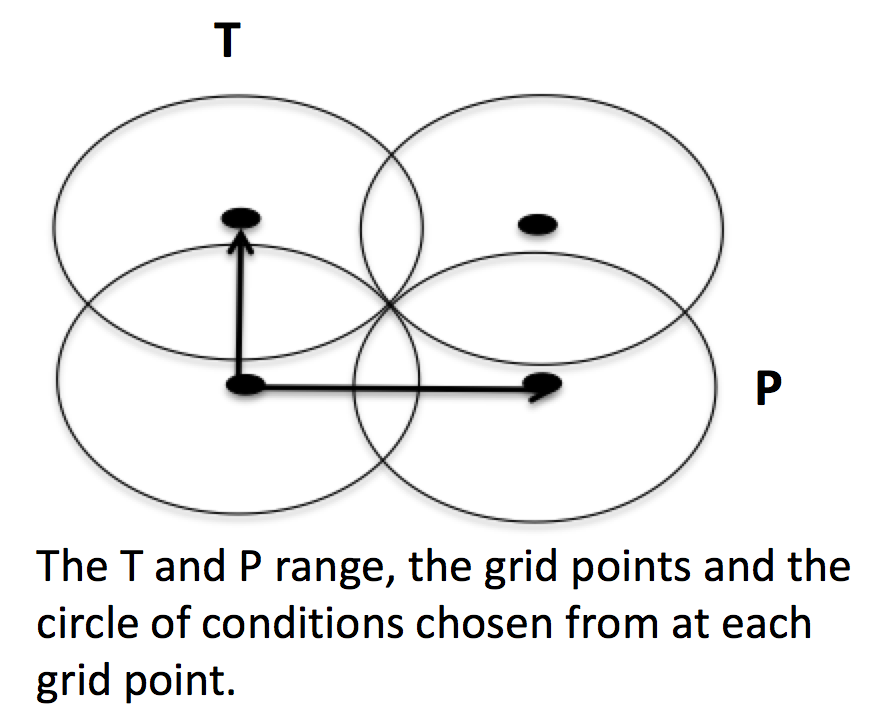
Under this setting rather than using reactors at fixed points, reaction conditions are sampled from a range of conditions. Conditions are chosen using a weighted stochastic grid sampling algorithm. An implemented objective function measures how desirable it is to sample from a point condition (T, P, concentrations) based on prior run conditions (weighted by how recent they were and how many objects they returned). Each iteration this objective function is evaluated at a grid of points spaning the reactor range (the grid has 20^N points where N is the number of dimensions). The grid values are then normalized to one and a grid point is chosen with probability equal to its normalized objective function value. Then a random step of maximum length sqrt(2)/2 times the distance between grid points is taken from that grid point to give the chosen condition point. The random numbers are seeded so that this does not make the algorithm non-deterministic.
These variable condition reactors run a defined number of times (nSims) each reactor cycle. Use of these reactors tends to
improve treatment of reaction conditions that otherwise would be between reactors and reduce the number of simulations needed by
focusing on reaction conditions at which the model terminates earlier. An example with sensitivity analysis at a specified reaction condition
is available below:
simpleReactor(
        temperature=[(1000,'K'),(1500,'K')],
        pressure=[(1.0,'bar'),(10.0,'bar')],
        nSims=12,
        initialMoleFractions={
        "ethane": [0.05,0.15],
        "O2": 0.1,
        "N2": 0.9,
        },
        terminationConversion={
        'ethane': 0.1,
        },
        terminationTime=(1e1,'s'),
        sensitivityTemperature = (1000,'K'),
        sensitivityPressure = (10.0,'bar'),
        sensitivityMoleFractions = {"ethane":0.1,"O2":0.9},
        sensitivity=["ethane","O2"],
        sensitivityThreshold=0.001,
        balanceSpecies = "N2",
        )
Note that increasing nSims improves convergence over the entire range, but convergence is only guaranteed at the
last set of nSims reaction conditions. Theoretically if nSims is set high enough the RMG model converges over the
entire interval. Except at very small values for nSims the convergence achieved is usually as good or superior to
that achieved using the same number of evenly spaced fixed reactors.
If there is a particular reaction condition you expect to converge more slowly than the rest of the range there is virtually no cost to using a single condition reactor (or a ranged reactor at a smaller range) at that condition and a ranged reactor with a smaller value for nSims. This is because the fixed reactor simulations will almost always be useful and keep the overall RMG job from terminating while the ranged reactor samples the faster converging conditions.
What you should actually set nSims to is very system dependent. The value you choose should be at least 2 + N
where N is the number of dimensions the reactor spans (T=>N=1, T and P=>N=2, etc…). There may be benefits to setting it as high
as 2 + 5N. The first should give you convergence over most of the interval that is almost always better than the same
number of fixed reactors. The second should get you reasonably close to convergence over the entire range for N <= 2.
For gas phase reactors if normalization of the ranged mole fractions is undesirable (eg. perhaps a specific species mole
fractions needs to be kept constant) one can use a balanceSpecies. When a balanceSpecies is used instead of
normalizing the mole fractions the concentration of the defined balanceSpecies is adjusted to maintain an overall mole
fraction of one. This ensures that all species except the balanceSpecies have mole fractions within the range specified.
4.6. Simulator Tolerances
The next two lines specify the absolute and relative tolerance for the ODE solver, respectively. Common values for the absolute tolerance are 1e-15 to 1e-25. Relative tolerance is usually 1e-4 to 1e-8:
simulator(
    atol=1e-16,
    rtol=1e-8,
    sens_atol=1e-6,
    sens_rtol=1e-4,
)
The sens_atol and sens_rtol are optional arguments for the sensitivity absolute tolerance and sensitivity relative tolerances, respectively. They
are set to a default value of 1e-6 and 1e-4 respectively unless the user specifies otherwise. They do not apply when sensitivity analysis is not conducted.
4.7. Model Tolerances
Model tolerances dictate how species get included in the model. For more information, see the theory behind how RMG builds models using the Flux-based Algorithm.
For running an initial job, it is recommended to only change the toleranceMoveToCore and toleranceInterruptSimulation values to an equivalent desired value. We find
that typically a value between 0.01 and 0.05 is best. If your model cannot converge within a few hours, more advanced settings such as reaction filtering
or pruning can be turned on to speed up your simulation at a slight risk of omitting chemistry.
            model(
    toleranceMoveToCore=0.1,
    toleranceInterruptSimulation=0.1,
)
toleranceMoveToCoreindicates how high the edge flux ratio for a species must get to enter the core model. This tolerance is designed for controlling the accuracy of final model.toleranceInterruptSimulationindicates how high the edge flux ratio must get to interrupt the simulation (before reaching theterminationConversionorterminationTime). This value should be set to be equal totoleranceMoveToCoreunless the advanced pruning feature is desired.
4.7.1. Advanced Setting: Branching Criterion
The flux criterion works very well for identifying new species that have high flux and therefore pathways that have high throughput flux. However, there are many important low flux pathways particularly those that result in net production of radicals such as chain branching reactions in combustion. Picking up these pathways with the flux criterion is difficult and almost always requires an appreciably lower flux tolerance that would otherwise be necessary causing RMG to pickup many unimportant species. The Branching criterion identifies important edge reactions based on the impact they are expected to have on the concentrations of core species. The branching specific tolerances shown in the example below are the recommended tolerances. These tolerances are much less system dependent than the flux tolerance and the recommended values are usually sufficient.
For example
model(
                toleranceMoveToCore=0.1,
                toleranceBranchReactionToCore=0.001,
          branchingIndex=0.5,
          branchingRatioMax=1.0,
)
4.7.2. Advanced Setting: Deadend Radical Elimination (RMS Reactors only)
When generating mechanisms involving significant molecular growth (such as in polymerization), there are many possible radicals, so fast propagation pathways compete with very slow termination and chain transfer reactions. These slow reactions individually usually have a negligible impact on the model, and thus will not be picked up by the flux or branching criteria. However, together they can have a very significant impact on the overall radical concentration, and need to be included in the generated mechanism. The deadend radical elimination algorithm identifies important chain transfer and termination reactions in the edge, based on their flux ratio with radical consumption and termination reactions in the core.
For example
model(
                toleranceMoveToCore=0.01,
                toleranceReactionToCoreDeadendRadical=0.01,
)
4.7.3. Advanced Setting: Radical Flux Criterion (RMS Reactors Only)
At high radical concentrations important products can accumulate from termination reactions. In these cases the flux and branching criteria can have difficulty adding in all of the important throughput terminations. For this case we have added a radical specific flux criterion. This criterion is similar to the flux criterion except that it looks at the net radical flux produced by each edge reaction instead of the total flux to each edge species.
For example
model(
                toleranceMoveToCore=0.1,
                toleranceRadMoveToCore=0.2,
)
4.7.4. Advanced Setting: Transitory Edge Analysis (RMS Reactors Only)
Suppose you are interested in the chemistry of a particular chemical species in your system. If that species is not high flux or participates in important branching reactions it may not be resolved accurately with the flux and branching criteria. Transitory edge analysis applies transitory sensitivity analysis to the edge of the mechanism to generate much more sophisticated information than the flux and branching algorithms can provide. This can be used to identify how edge reactions are likely to affect the concentrations of non-participant core species. By applying this analysis to a given target species we can add all edge reactions that the target species is sensitive to above a given tolerance. This criterion is highly effective, but it can also be very computationally expensive for models with large edges. One can reduce the computational cost by increasing the transitoryStepPeriod, which is the number of solver time steps RMG takes between transitory edge analyses. how
For example
model(
                toleranceMoveToCore=0.1,
                toleranceTransitoryDict={"NO":0.2},
                transitoryStepPeriod=20,
)
4.7.5. Advanced Setting: Speed Up By Filtering Reactions
For generating models for larger molecules, RMG-Py may have trouble converging because it must find reactions on the order of \((n_{reaction\: sites})^{{n_{species}}}\). Thus it can be further sped up by pre-filtering reactions that are added to the model. This modification to the algorithm does not react core species together until their concentrations are deemed high enough. It is recommended to turn on this flag when the model does not converge with normal parameter settings. See Filtering Reactions within the Flux-based Algorithm. for more details.
model(
          toleranceMoveToCore=0.1,
          toleranceInterruptSimulation=0.1,
          filterReactions=True,
          filterThreshold=5e8,
)
Additional parameters:
filterReactions: set toTrueif reaction filtering is turned on. By default it is set to False.filterThreshold: click here for more description about its effect. Default:5e8
4.7.6. Advanced Setting: Speed Up by Pruning
For further speed-up, it is also possible to perform mechanism generation with pruning of “unimportant” edge species to reduce memory usage.
A typical set of parameters for pruning is:
model(
    toleranceMoveToCore=0.5,
    toleranceInterruptSimulation=1e8,
    toleranceKeepInEdge=0.05,
    maximumEdgeSpecies=200000,
    minCoreSizeForPrune=50,
    minSpeciesExistIterationsForPrune=2,
    )
Additional parameters:
toleranceKeepInEdgeindicates how low the edge flux ratio for a species must be to keep on the edge. This should be set to zero, which is its default.maximumEdgeSpeciesindicates the upper limit for the size of the edge. The default value is set to1000000species.minCoreSizeForPruneensures that a minimum number of species are in the core before pruning occurs, in order to avoid pruning the model when it is far away from completeness. The default value is set to 50 species.minSpeciesExistIterationsForPruneis set so that the edge species stays in the job for at least that many iterations before it can be pruned. The default value is 2 iterations.
Recommendations:
We recommend setting toleranceKeepInEdge to not be larger than 10% of toleranceMoveToCore, based on a pruning case study.
In order to always enable pruning, toleranceInterruptSimulation should be set as a high value, e.g. 1e8.
maximumEdgeSpecies can be adjusted based on user’s RAM size. Usually 200000 edge species would cause memory shortage of 8GB computer,
setting maximumEdgeSpecies = 200000 (or lower values) could effectively prevent memory crash.
Additional Notes:
Note that when using pruning, RMG will not prune unless all reaction systems reach the goal reaction time or conversion without exceeding the toleranceInterruptSimulation.
Therefore, you may find that RMG is not pruning even though the model edge size exceeds maximumEdgeSpecies, or an edge species has flux below the toleranceKeepInEdge. This is
a safety check within RMG to ensure that species are not pruned too early, resulting in inaccurate chemistry. In order to increase the likelihood of pruning you can
try increasing toleranceInterruptSimulation to an arbitrarily high value.
As a contrast, a typical set of parameters for non-pruning is:
model(
    toleranceKeepInEdge=0,
    toleranceMoveToCore=0.5,
    toleranceInterruptSimulation=0.5,
)
where toleranceKeepInEdge is always 0, meaning all the edge species will be kept in edge since all the edge species have positive flux.
toleranceInterruptSimulation equals to toleranceMoveToCore so that ODE simulation get interrupted once discovering a new core species.
Because the ODE simulation is always interrupted, no pruning is performed.
Please find more details about the theory behind pruning at Pruning Theory.
4.7.7. Advanced Setting: Thermodynamic Pruning
Thermodynamic pruning is an alternative to flux pruning that does not require a given simulation to complete to remove excess species. The thermodynamic criteria is calculated by determining the minimum and maximum Gibbs energies of formation (Gmin and Gmax) among species in the core. If the Gibbs energy of formation of a given species is G the value of the criteria is (G-Gmax)/(Gmax-Gmin). All of the Gibbs energies are evaluated at the highest temperature used in all of the reactor systems. This means that a value of 0.2 for the criterion implies that it will not add species that have Gibbs energies of formation greater than 20% of the core Gibbs energy range greater than the maximum Gibbs energy of formation within the core.
For example
model(
    toleranceMoveToCore=0.5,
    toleranceInterruptSimulation=0.5,
    toleranceThermoKeepSpeciesInEdge=0.5,
    maximumEdgeSpecies=200000,
    minCoreSizeForPrune=50,
    )
Advantages over flux pruning:
Species are removed immediately if they violate tolerance
Completing a simulation is unnecessary for this pruning so there is no need
to waste time setting the interrupt tolerance higher than the movement tolerance.
Will always maintain the correct maximumEdgeSpecies.
Primary disadvantage:
Since we determine whether to add species primarily based on flux, at tight tolerances this is more likely to kick out species RMG might otherwise have added to core.
4.7.8. Advanced Setting: Taking Multiple Species At A Time
Taking multiple objects (Species, Reaction or PDepNetwork) during a given simulation can often decrease your overall model generation time
over only taking one. For this purpose there is a maxNumObjsPerIter parameter that allows RMG to take
that many Species, Reaction or PDepNetwork from a given simulation. This is done in the order they trigger their respective criteria.
You can also set terminateAtMaxObjects=True to cause it to terminate when it has the maximum
number of objects allowed rather than waiting around until it hits an interrupt tolerance. This
avoids additional simulation time, but will also make it less likely to finish simulations, which can
affect flux pruning.
For example
model(
        toleranceKeepInEdge=0.0,
        toleranceMoveToCore=0.1,
        toleranceInterruptSimulation=0.3,
        maxNumObjsPerIter=2,
        terminateAtMaxObjects=True,
)
Note that this can also result in larger models, however, sometimes these larger models (from taking more than one object at a time) pick up chemistry that would otherwise have been missed.
4.7.9. Advanced Settings: Other
dynamicsTimeScale: The time before which the dynamics criterion cannot be used to bring reactions into the model. This is useful because the math behind the dynamics criterion breaks down astapproaches 0, thus restricting the use of the dynamics criterion until later times may reduce the number of junk species/reactions added to the model.ignoreOverallFluxCriterion: Causes RMG to use the given flux criterion only for determining if aPDepNetworkshould be explored and not whether species should enter the model. Lets you run pressure dependence alongside the dynamics criterion without the flux criterion.
4.8. On the fly Quantum Calculations
This block is used when quantum mechanical calculations are desired to determine thermodynamic parameters.
These calculations are only run if the molecule is not included in a specified thermo library.
The onlyCyclics option, if True, only runs these calculations for cyclic species.
In this case, group additive estimates are used for all other species.
Molecular geometries are estimated via RDKit [RDKit]. Either MOPAC (2009 and 2012) or GAUSSIAN (2003 and 2009) can be used with the semi-empirical pm3, pm6, and pm7 (pm7 only available in MOPAC2012), specified in the software and method blocks. A folder can be specified to store the files used in these calculations, however if not specified this defaults to a QMfiles folder in the output folder.
The calculations are also only run on species with a maximum radical number set by the user. If a molecule has a higher radical number, the molecule is saturated with hydrogen atoms, then quantum mechanical calculations with subsequent hydrogen bond incrementation is used to determine the thermodynamic parameters.
The following is an example of the quantum mechanics options
quantumMechanics(
        software='mopac',
        method='pm3',
        fileStore='QMfiles',
        scratchDirectory = None,
        onlyCyclics = True,
        maxRadicalNumber = 0,
        )
RDKit: Open-source cheminformatics; http://www.rdkit.org
4.9. Machine Learning-based Thermo Estimation
This block is used to turn on the machine learning module to estimate thermodynamic parameters. These calculations are only run if the molecule is not included in a specified thermo library. There are a number of different settings that can be specified to tune the estimator so that it only tries to estimate some species. This is useful because the machine learning model may perform poorly for some molecules and group additivity may be more suitable. Using the machine learning estimator for fused cyclic species of moderate size or any species with significant proportions of oxygen and/or nitrogen atoms will most likely yield better estimates than group additivity.
The available options with their default values are
mlEstimator(
    thermo=True,
    name='main',
    minHeavyAtoms=1,
    maxHeavyAtoms=None,
    minCarbonAtoms=0,
    maxCarbonAtoms=None,
    minOxygenAtoms=0,
    maxOxygenAtoms=None,
    minNitrogenAtoms=0,
    maxNitrogenAtoms=None,
    onlyCyclics=False,
    onlyHeterocyclics=False,
    minCycleOverlap=0,
    H298UncertaintyCutoff=(3.0, 'kcal/mol'),
    S298UncertaintyCutoff=(2.0, 'cal/(mol*K)'),
    CpUncertaintyCutoff=(2.0, 'cal/(mol*K)')
)
name is the name of the folder containing the machine learning model architecture and parameters in the RMG
database. The next several options allow setting limits on the numbers of atoms. onlyCyclics means that only cyclic
species will be estimated. onlyHeterocyclics means that only heterocyclic species will be estimated. Note that
if onlyHeterocyclics setting is set to True, the machine learning estimator will be restricted to heterocyclic
species regardless of the onlyCyclics setting. If onlyCyclics is False and onlyHeterocyclics is True,
RMG will log a warning that onlyCyclics should also be True and the machine learning estimator will be
restricted to heterocyclic species because they are a subset of cyclics.
minCycleOverlap specifies the minimum number of atoms that must be shared between any two cycles. For example,
if there are only disparate monocycles or no cycles in a species, the overlap is zero; “spiro” cycles have an overlap
of one; “fused” cycles have an overlap of two; and “bridged” cycles have an overlap of at least three. Note that
specifying any value greater than zero will automatically restrict the machine learning estimator to only consider
cyclic species regardless of the onlyCyclics setting. If onlyCyclics is False and minCycleOverlap is greater
than zero, RMG will log a warning that onlyCyclics should also be True and the machine learning estimator will be
restricted to only cyclic species with the specified minimum cycle overlap.
Note that the current machine learning model is not yet capable of estimating uncertainty so the UncertaintyCutoff
values do not yet have any effect.
4.10. Pressure Dependence
This block is used when the model should account for pressure
dependent rate coefficients. RMG can estimate pressure dependence kinetics based on Modified Strong Collision and Reservoir State methods.
The former utilizes the modified strong collision approach of Chang, Bozzelli, and Dean [Chang2000],
and works reasonably well while running more rapidly. The latter
utilizes the steady-state/reservoir-state approach of Green and Bhatti [Green2007],
and is more theoretically sound but more expensive.
The following is an example of pressure dependence options
pressureDependence(
        method='modified strong collision',
        maximumGrainSize=(0.5,'kcal/mol'),
        minimumNumberOfGrains=250,
        temperatures=(300,2000,'K',8),
        pressures=(0.01,100,'bar',5),
        interpolation=('Chebyshev', 6, 4),
        maximumAtoms=16,
)
The various options are as follows:
4.10.1. Method used for estimating pressure dependent kinetics
To specify the modified strong collision approach, this item should read
method='Modified Strong Collision'
To specify the reservoir state approach, this item should read
method='Reservoir State'
For more information on the two methods, consult the following resources :
A.Y. Chang, J.W. Bozzelli, and A. M. Dean. “Kinetic Analysis of Complex Chemical Activation and Unimolecular Dissociation Reactions using QRRK Theory and the Modified Strong Collision Approximation.” Z. Phys. Chem. 214 (11), p. 1533-1568 (2000).
N.J.B. Green and Z.A. Bhatti. “Steady-State Master Equation Methods.” Phys. Chem. Chem. Phys. 9, p. 4275-4290 (2007).
4.10.2. Grain size and minimum number of grains
Since the \(k(E)\) requires discretization in the energy space, we need to specify the number of energy grains to use when solving the Master Equation. The default value for the minimum number of grains is 250; this was selected to balance the speed and accuracy of the Master Equation solver method. However, for some pressure-dependent networks, this number of energy grains will result in the pressure-dependent \(k(T, P)\) being greater than the high-P limit
maximumGrainSize=(0.5,'kcal/mol')
minimumNumberOfGrains=250
4.10.3. Temperature and pressure for the interpolation scheme
To generate the \(k(T,P)\) interpolation model, a set of temperatures and pressures must be used. RMG can do this automatically, but it must be told a few parameters. We need to specify the limits of the temperature and pressure for the fitting of the interpolation scheme and the number of points to be considered in between this limit. For typical combustion model temperatures of the experiments range from 300 - 2000 K and pressure 1E-2 to 100 bar
temperatures=(300,2000,'K',8)
pressures=(0.01,100,'bar',5)
4.10.4. Interpolation scheme
To use logarithmic interpolation of pressure and Arrhenius interpolation for temperature, use the line
interpolation=('PDepArrhenius',)
The auxillary information printed to the Chemkin chem.inp file will have the “PLOG”
format. Refer to Section 3.5.3 of the CHEMKIN_Input.pdf document and/or
Section 3.6.3 of the CHEMKIN_Theory.pdf document. These files are part of
the CHEMKIN manual.
To fit a set of Chebyshev polynomials on inverse temperature and logarithmic pressure axes mapped to [-1,1], specify ‘’Chebyshev’ interpolation. You should also specify the number of temperature and pressure basis functions by adding the appropriate integers. For example, the following specifies that six basis functions in temperature and four in pressure should be used
interpolation=('Chebyshev', 6, 4)
The auxillary information printed to the Chemkin chem.inp file will have the “CHEB”
format. Refer to Section 3.5.3 of the CHEMKIN_Input.pdf document and/or
Section 3.6.4 of the CHEMKIN_Theory.pdf document.
Regarding the number of polynomial coeffients for Chebyshev interpolated rates,
plese refer to the rmgpy.kinetics.Chebyshev documentation.
The number of pressures and temperature coefficents should always be smaller
than the respective number of user-specified temperatures and pressures.
4.10.5. Maximum size of adduct for which pressure dependence kinetics be generated
By default pressure dependence is run for every system that might show pressure dependence, i.e. every isomerization, dissociation, and association reaction. In reality, larger molecules are less likely to exhibit pressure-dependent behavior than smaller molecules due to the presence of more modes for randomization of the internal energy. In certain cases involving very large molecules, it makes sense to only consider pressure dependence for molecules smaller than some user-defined number of atoms. This is specified e.g. using the line
maximumAtoms=16
to turn off pressure dependence for all molecules larger than the given number of atoms (16 in the above example).
4.10.6. Completed Pressure-Dependent Networks
Sometimes you have a pressure-dependent network that has been studied in great detail and included in a seed mechanism or reaction library (such as CH2O2), and you don’t want RMG to add additional reactions to that network. Adding RMG’s estimates to a thoroughly studied network will likely make your model worse, as the original authors would have included any important reactions.
You can specify that certain networks should not be expanded further using the
completedNetworks parameter within the pressureDependence() block. This
parameter takes a list of chemical formulas identifying the networks that should
be considered complete. For example:
pressureDependence(
    method='modified strong collision',
    maximumGrainSize=(0.5,'kcal/mol'),
    minimumNumberOfGrains=250,
    temperatures=(300,2000,'K',8),
    pressures=(0.01,100,'bar',5),
    interpolation=('Chebyshev', 6, 4),
    maximumAtoms=16,
    completedNetworks=['CH2O2'],
)
Multiple networks can be specified in the list:
completedNetworks=['CH2O2', 'C2H6'],
When a network is marked as completed, RMG will not add any new reactions to it, though reactions already present in seed mechanisms will still be used.
4.11. Uncertainty Analysis
It is possible to request automatic uncertainty analysis following the convergence of an RMG simulation by including an uncertainty options block in the input file:
uncertainty(
    localAnalysis=False,
    globalAnalysis=False,
    uncorrelated=True,
    correlated=True,
    localNumber=10,
    globalNumber=5,
    terminationTime=None,
    pceRunTime=1800,
    pceErrorTol=None,
    pceMaxEvals=None,
    logx=True
)
RMG can perform local uncertainty analysis using first-order sensitivity coefficients output by the native RMG solver.
This is enabled by setting localAnalysis=True. Performing local uncertainty analysis requires suitable settings in
the reactor block (see Reaction System). At minimum, the output species to perform sensitivity analysis on must
be specified, via the sensitivity argument. RMG will then perform local uncertainty analysis on the same species.
Species and reactions with the largest sensitivity indices will be reported in the log file and output figures.
The number of parameters reported can be adjusted using localNumber.
RMG can also perform global uncertainty analysis, implemented using Cantera [Cantera] and the MIT Uncertainty
Quantification (MUQ) [MUQ] library. This is enabled by setting globalAnalysis=True. Note that local analysis
is a required prerequisite of running the global analysis (at least for this semi-automatic approach), so
localAnalysis will be enabled regardless of the input file setting. The analysis is performed by allowing the
input parameters with the largest sensitivity indices (as determined from the local uncertainty analysis) to vary
while performing reactor simulations using Cantera. MUQ is used to fit a Polynomial Chaos Expansion (PCE) to the
resulting output surface. The number of input parameters chosen can be adjusted using globalNumber.
Note that this number applies independently to thermo and rate parameters and output species.
For example globalNumber=5 for analysis on a single output species will result in 10 parameters being varied, while
having two output species could result in up to 20 parameters being varied, assuming no overlap in the sensitive input
parameters for each output.
The uncorrelated and correlated options refer to two approaches for uncertainty analysis. Uncorrelated means
that all input parameters are considered to be independent, each with their own uncertainty bounds. Thus, the output
uncertainty distribution is determined on the basis that every input parameter could vary within the full range of
its uncertainty bounds. Correlated means that inherent relationships between parameters (such as rate rules for kinetics
or group additivity values for thermochemistry) are accounted for, which reduces the uncertainty space of the input
parameters.
Finally, there are a few miscellaneous options for global uncertainty analysis. The terminationTime applies for the
reactor simulation. It is only necessary if termination time is not specified in the reactor settings (i.e. only other
termination criteria are used). For PCE generation, there are three termination options: pceRunTime sets a time
limit for adapting the PCE to the output, pceErrorTol sets the target L2 error between the PCE model and the true
output, and pceMaxEvals sets a limit on the total number of model evaluations used to adapt the PCE.
Longer run time, smaller error tolerance, and more model evaluations all contribute to more accurate results at the
expense of computation time. The logx option toggles the output parameter space between mole fractions and log mole
fractions. Results in mole fraction space are more physically meaningful, while results in log mole fraction space can
be directly compared against local uncertainty results.
Important Note: The current implementation of uncertainty analysis assigns values for input parameter uncertainties based on the estimation method used by RMG. Actual uncertainties associated with the original data sources are not used. Thus, the output uncertainties reported by these analyses should be viewed with this in mind.
The uncertainty analysis is described in [Gao2016thesis] and [Gao2020].
Goodwin, D.G.; Moffat, H.K.; Speth, R.L. Cantera: An object-oriented software toolkit for chemical kinetics, thermodynamics, and transport processes; https://www.cantera.org/
Conrad, P.R.; Parno, M.D.; Davis, A.D.; Marzouk, Y.M. MIT Uncertainty Quantification Library (MUQ); http://muq.mit.edu/
Gao, C. W.; Ph.D. Thesis. 2016.
Gao, CW; Liu, M; Green, WH. Uncertainty analysis of correlated parameters in automated reaction mechanism generation. Int J Chem Kinet. 2020; 52: 266– 282. https://doi.org/10.1002/kin.21348
4.12. Miscellaneous Options
Miscellaneous options:
options(
    name='Seed',
    generateSeedEachIteration=True,
    saveSeedToDatabase=True,
    units='si',
    generateOutputHTML=True,
    generatePlots=False,
            generatePESDiagrams=False,
    saveSimulationProfiles=True,
    verboseComments=False,
    saveEdgeSpecies=True,
    keepIrreversible=True,
    trimolecularProductReversible=False,
    saveSeedModulus=-1
)
The name field is the name of any generated seed mechanisms
Setting generateSeedEachIteration to True (default) tells RMG to save and update a seed mechanism and thermo library during the current run
Setting saveSeedToDatabase to True tells RMG (if generating a seed) to also save that seed mechanism and thermo library directly into the database
The units field is set to si. Currently there are no other unit options.
Setting generateOutputHTML to True will let RMG know that you want to save 2-D images (png files in the local species folder) of all species in the generated core model. It will save a visualized
HTML file for your model containing all the species and reactions. Turning this feature off by setting it to False may save memory if running large jobs.
Setting generatePlots to True will generate a number of plots describing the statistics of the RMG job, including the reaction model core and edge size and memory use versus execution time. These will be placed in the output directory in the plot/ folder.
Setting generatePESDiagrams to True will generate potential energy surface diagrams for each pressure dependent network in the model. These diagrams will be saved in the pdep/ folder in the output directory. Only applicable if pressure dependence is enabled.
Setting saveSimulationProfiles to True will make RMG save csv files of the simulation in .csv files in the solver/ folder. The filename will be simulation_1_26.csv where the first number corresponds to the reaciton system, and the second number corresponds to the total number of species at the point of the simulation. Therefore, the highest second number will indicate the latest simulation that RMG has complete while enlarging the core model. The information inside the csv file will provide the time, reactor volume in m^3, as well as mole fractions of the individual species.
Setting verboseComments to True will make RMG generate chemkin files with complete verbose commentary for the kinetic and thermo parameters. This will be helpful in debugging what values are being averaged for the kinetics. Note that this may produce very large files.
Setting saveEdgeSpecies to True will make RMG generate chemkin files of the edge reactions in addition to the core model in files such as chem_edge.inp and chem_edge_annotated.inp files located inside the chemkin folder. These files will be helpful in viewing RMG’s estimate for edge reactions and seeing if certain reactions one expects are actually in the edge or not.
Setting keepIrreversible to True will make RMG import library reactions as is, whether they are reversible or irreversible in the library. Otherwise, if False (default value), RMG will force all library reactions to be reversible, and will assign the forward rate from the relevant library.
Setting trimolecularProductReversible to False will not allow families with three products to react in the reverse direction. Default is True.
Setting saveSeedModulus to -1 will only save the seed from the last iteration at the end of an RMG job. Alternatively, the seed can be saved every n iterations by setting saveSeedModulus to n.
4.13. Species Constraints
RMG can generate mechanisms with a number of optional species constraints, such as total number of carbon atoms or electrons per species. These are applied to all of RMG’s reaction families.
generatedSpeciesConstraints(
    allowed=['input species','seed mechanisms','reaction libraries'],
    maximumCarbonAtoms=10,
    maximumOxygenAtoms=2,
    maximumNitrogenAtoms=2,
    maximumSiliconAtoms=2,
    maximumSulfurAtoms=2,
    maximumHeavyAtoms=10,
    maximumSurfaceSites=2,
            maximumSurfaceBondOrder=4,
    maximumRadicalElectrons=2,
    maximumSingletCarbenes=1,
    maximumCarbeneRadicals=0,
    maximumIsotopicAtoms=2,
    allowSingletO2 = False,
    speciesCuttingThreshold=20,
)
An additional flag allowed can be set to allow species
from either the input file, seed mechanisms, or reaction libraries to bypass these constraints.
Note that this should be done with caution, since the constraints will still apply to subsequent
products that form.
By default, the allowSingletO2 flag is set to False. See Representing Oxygen for more information.
Note that speciesCuttingThreshold is set by default to 20 heavy atoms. This means that if a species containing
20 or more heavy atoms is generated, it will be automatically split into fragments to save computational resources.
If fragments are not desired, the speciesCuttingThreshold may be set to an arbitrarily large number.
4.14. Staging
It is now possible to concatenate different model and simulator blocks into the same run in stages. Any given stage will terminate when the RMG run terminates and then the current group of model and simulator parameters will be switched out with the next group and the run will continue until that stage terminates. Once the last stage terminates the run ends normally. This is currently enabled only for the model and simulator blocks.
There must be the same number of each of these blocks (although only having one simulator block and many model blocks is enabled as well) and RMG will enter each stage these define in the order they were put in the input file.
To enable easier manipulation of staging a new parameter in the model block was developed maxNumSpecies that is the number of core species at which that stage (or if it is the last stage the entire model generation process) will terminate.
For example
model(
        toleranceKeepInEdge=0.0,
        toleranceMoveToCore=0.1,
        toleranceInterruptSimulation=0.1,
        maximumEdgeSpecies=100000,
        maxNumSpecies=100
)
4.15. Restarting from a Seed Mechanism
The only method for restarting an RMG-Py job is to restart the job from a seed mechanism. There are many scenarios when the user might want to do this, including continuing on a job that ran out of time or crashed as the result of a now fixed bug. To restart from a seed mechanism, the block below must be added on to the input file.
restartFromSeed(path='seed')
The path flag is the path to the seed mechanism folder, which contains three subfolders that must be titled as
follows: filters, seed, seed_edge. The path can be a relative path from the input.py file or an absolute path on disk
Alternatively, you may also specify the paths to each of the following files/directories: coreSeed (path to seed
mechanism folder containing files named reactions.py and `dictionary.txt` that will go into the model core),
edgeSeed (path to edge seed mechanism folder containing files named reactions.py and `dictionary.txt` that will
go into the model edge), filters (an h5 binary file storing the uni-, bi-, and optionally tri-molecular thresholds
generated by RMG from previous run (must be RMG version > 2.4.1)), speciesMap (a YAML file specifying what species are
at each index in the filters).
restartFromSeed(coreSeed='seed/seed'  # Path to core seed folder. Must contain `reactions.py` and `dictionary.txt`
                edgeSeed='seed/seed_edge'  # Path to edge seed folder containing `reactions.py` and `dictionary.txt`
                filters='seed/filters/filters.h5',
                speciesMap='seed/filters/species_map.yml')
Then, to restart from the seed mechanism the input file is submitted as normal.
python rmg.py input.py
Once the restart job has begun, RMG will move the seed mechanism files to a new subfolder in the output directory
entitled previous_restart. This is to back-up the seed mechanism used for restarting, as everything in the seed
subfolder of the output directory is overwritten by RMG during the course of mechanism generation.
RMG also outputs a file entitled restart_from_seed.py the first time a seed mechanism is generated during the course
of an RMG job (so long as the RMG job was not itself a restarted job). This file is an exact duplicate of the original
input file with the exception that the restart block has been added on automatically for convenience. In this way this
file is treated in the exact way as a normal input file.
Finally, note that it is advised to turn on generating the seed each iteration so that you can restart an RMG job right where it left off.
This can be done by setting generateSeedEachIteration=True in the options block of the input file.